 |
BIOL 4120 Principles of Ecology |
| Opuntia cactus on a Canaveral sand dune | |
|
BIOL 4120 Principles of Ecology |
| Opuntia cactus on a Canaveral sand dune | |
Effective Population Size
Worksheet
Back to:
| Course Page | Tennessee State Home page |
| Bio 412 Page | Ganter home page |
The material on this page is also covered in the notes on population biology
Effective Population Size when the population sex ration differs from 1:1
When there are unequal numbers of each sex, random error will be more influential in the rarer sex. If you report only the population size, it is usually assumed that the population is 50% male and 50% female. This is the most common situation. Consider, however, two populations: one with 100 of each sex and the other with 20 males and 180 females. The next generation will receive 50% of its genes from each sex, no matter what the sex ratio is. In the first population, 100 males contribute and random error in the transmission of alleles to the next generation happen at a rate appropriate for a population of that size. In the other population, there are only 10 males, and random events are much more likely to influence which alleles get passed to the next generation. You might argue that this effect is countered by the larger female population -- 180 versus 100. However, the effects are not symmetric. The male ratio (10 males to 100 males) is not the reciprocal of the female ratio (180 females to 100) and the influence of the change in male population is not completely offset by the greater number of females.
This means that we can't compare the effect of genetic drift in different populations unless they both have the same sex ratio. This is OK, because there is a way to adjust for the effect of an excess of males or females. What we do is to calculate the size of a population that has a 1 to 1 sex ratio, but is equally prone to the influence of genetic drift as is the population with a unequal sex ratio. This population size is called the effective population size, and we can compare any two effective population sizes because they all are assumed to have a 1 to 1 sex ratio.
We will calculate the effects in the problems below. If you want to check your answers, send me an email, come into the office, or call. I'll give you my solutions and discuss any problems you might have.
Formula
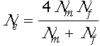
Ne is the effective population size
Nf is the number of females
Nm is the number of males
As an exercise in calculating the effect, you should fill in this table (remember how computer savvy you are now) and construct a graph of Ne versus the sex ratio. The sex ratio can be either males divided by females or females divided by males. I used the first ratio when I did this problem.
| Number of Males | Number of Females | sex ratio m/f |
4NmNf | Nm+Nf | Ne |
| 100 | 100 | ||||
| 90 | 110 | ||||
| 80 | 120 | ||||
| 70 | 130 | ||||
| 60 | 140 | ||||
| 50 | 150 | ||||
| 40 | 160 | ||||
| 30 | 170 | ||||
| 20 | 180 | ||||
| 10 | 190 | ||||
| 5 | 195 | ||||
| 1 | 199 |
Effective Population Size when the population size varies from year to year
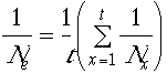
A second instance in which one can't simply calculate the effect of genetic drift is when a population is fluctuating in size. In the years when the population is small, the effect is large and when the population gets large, the influence of genetic drift is small. So, how is one to judge the overall effect. This involves and averaging of population sized. However, we have that same asymmetric effect as above. Little numbers count more. When you calculate the average (called the arithmetic mean), big and little sizes have the same influence. This means that we have to look for a mean that gives more weight to small than large size. This mean is called the Harmonic Mean and is calculated as the reciprocal. I give you the formula here from the notes and then an easier formula (a simple algebraic rearrangement of the previous formula).
As presented
Rearranged:
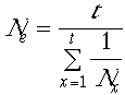
Ne is the effective population size for the entire period
Nt is the population size at a particular time
t is the number of times the population is sampled
Now, let's calculate the effect when there is no change in size:
| Sample (t) | Pop. Size (Nt) | 1/Nt |
| 1 | 500 | 0.002 |
| 2 | 500 | 0.002 |
| 3 | 500 | 0.002 |
| 4 | 500 | 0.002 |
| 5 | 500 | 0.002 |
| 6 | 500 | 0.002 |
| 7 | 500 | 0.002 |
| 8 | 500 | 0.002 |
| 9 | 500 | 0.002 |
| 10 | 500 | 0.002 |
| Total | 5000 | 0.02 |
| Arithmetic Mean | Effective Population Size (Ne) | |
| 500 | 500.000 |
Let's calculate it when there is one bad year, when only 50 are in the population:
| Sample (t) | Pop. Size (Nt) | 1/Nt |
| 1 | 50 | 0.02 |
| 2 | 500 | 0.002 |
| 3 | 500 | 0.002 |
| 4 | 500 | 0.002 |
| 5 | 500 | 0.002 |
| 6 | 500 | 0.002 |
| 7 | 500 | 0.002 |
| 8 | 500 | 0.002 |
| 9 | 500 | 0.002 |
| 10 | 500 | 0.002 |
| Total | 4550 | 0.038 |
| Arithmetic Mean | Effective Population Size (Ne) | |
| 455 | 263.158 |
You should try to calculate both the arithmetic mean and Ne to make sure you know how to do it. Notice the big gap between the two population sizes. The average greatly overestimates the size and will greatly underestimate the effect of genetic drift. Look at what happens when the population gets large for a year:
| Sample (t) | Pop. Size (Nt) | 1/Nt |
| 1 | 5000 | 0.0002 |
| 2 | 500 | 0.002 |
| 3 | 500 | 0.002 |
| 4 | 500 | 0.002 |
| 5 | 500 | 0.002 |
| 6 | 500 | 0.002 |
| 7 | 500 | 0.002 |
| 8 | 500 | 0.002 |
| 9 | 500 | 0.002 |
| 10 | 500 | 0.002 |
| Total | 9500 | 0.0182 |
| Arithmetic Mean | Effective Population Size (Ne) | |
| 950 | 549.451 |
As you can see, the arithmetic mean once again over estimates the effective population size over this time period and under estimates the importance of genetic drift. Finally, what is the effect of more variation than a single bad year. You can calculate this:
| Sample (t) | Pop. Size (Nt) | 1/Nt |
| 1 | 50 | |
| 2 | 50 | |
| 3 | 500 | |
| 4 | 500 | |
| 5 | 500 | |
| 6 | 500 | |
| 7 | 500 | |
| 8 | 500 | |
| 9 | 500 | |
| 10 | 500 | |
| Total | ||
| Arithmetic Mean | Effective Population Size (Ne) | |
Now, a last point. I have calculated the arithmetic mean and effective population size when you systematically add bad years. The results are in the table below. The first column is the number of bad years (with a value of 50) out of 10 total years. The years not bad have a population size of 500, as above. You should graph the arithmetic mean and effective population size versus the number of bad years to get a feel for how these two things relate to one another.
| Number of years with 50 | Arithmetic Mean | Ne |
| 1 | 455 | 263.158 |
| 2 | 410 | 178.571 |
| 3 | 365 | 135.135 |
| 4 | 320 | 108.696 |
| 5 | 275 | 90.909 |
| 6 | 230 | 78.125 |
| 7 | 185 | 68.493 |
| 8 | 140 | 60.976 |
| 9 | 95 | 54.945 |
| 10 | 50 | 50.000 |
Last updated on September 10, 1999