|
|
BIOL
4120
Principles of Ecology
Phil Ganter
320
Harned Hall
963-5782
|
The field
above has many species of plant, all with similar resource needs.
Could the field support more of each species or are numbers limited?
Are the plants competing? |
Lecture 13 Interspecific Competition
Email me
Back to:
Overview - Link
to Course
Objectives
Species
Interactions
This lecture begins a series of
lectures on species interactions. Below is a general scheme for those
interactions. Some are familiar, but others may new. The scheme
is based on whether the individual organisms involved in the interaction are
helped, hurt, or unaffected as a result of the interaction. You can see
that there are several +,- interactions
Hurt(-), helped(+), or not affected(0)
| Name of interaction |
Species A |
Species B |
| Mutualism* |
+
|
+
|
| Commensalism* |
+
|
0
|
| Competition |
-
|
-
|
| Allelopathy |
+
|
-
|
| Herbivory* |
+
|
-
|
| Predation |
+
|
-
|
| Parasitism* |
+
|
-
|
| Amensalism |
-
|
0
|
* symbiosis
(living in intimate contact) can occur in several of these interactions
- Mutualism, Commensalism, Herbivory and Parasitism can all involve symbiosis
- Amensalism
has been added for the interaction in which one species is hurt, but the other
does not benefit
- As wild pigs forage,
they often disturb the upper layer of soil and many organisms may be taken
from their burrows and exposed to predation by the action of the pigs,
although the harm that the burrowers suffer does not improve the pig's
situation at all.
- Allelopathy
refers to the release of toxins in to the environment. The term was
first applied to plant releases of toxins but toxin release has been found
by animals (sponge interactions), bacteria (bacteriocins), and fungi (mycosins),
so it is a widespread phenomenon.
- can be a situation
in which a species is hurt by the release of toxins but the species that
released the toxins gains no benefit (in which case it is amensalism)
- can be that the
species that releases the toxins does gain by their release, in which
case it becomes a mechanism for competition or predation avoidance.
Interspecific
Competition
Interspecific
versus intraspecific
- Review what was discussed
in Lecture 11 on intraspecific competition
- Interspecific Competition
arises out of the need for a scarce resource, just as intraspecific competition
does and the mechanism can be scramble or interference competition.
Lotka-Volterra
model of Interspecific
competition
- Based on the Logistic
model
- adds the presence
of another species or genotype to the braking effect of the population
being modeled
- now, the reduction
in the growth rate is the sum of the numbers of the two species present
- need a way to correct
for differences between species (see below)
- First, define the Lotka-Volterra
interaction coefficient or
 (the Greek letter alpha)

Interpretation
of a
- It is the effect an individual of
another species has on an individual of a competing species
of expressed as the equivalent number of the competing species.
- If species A eats three times what
species B does, then 5 individuals of species A would eat the
same as 15 individuals of species B and would be
3
- Next, we modify the
logistic by including the effect of the presence of one species on another,
using the relationship defined above
and
- So, what are the possible
outcomes predicted by these equations?
- Depending on the
values of K's and a's, they can predict either:
- Trivial equilibria
- Called trivial because they
predict an outcome that is obvious
- One species drives the other
out and you get the K number of the winning species
- either Species A or B remains
and the other goes locally extinct
- Stable equilibrium
- Displacing the system (adding
or removing individuals of one or both species) takes you back
to the same equilibrium point
- this predicts that both species
will continue to coexist in this environment indefinitely
- Unstable equilibrium
- Displacing the system takes
you to one of two possible outcomes:
- Species A wins
- Species B wins
- Which one occurs depends
on what sort of displacement takes place
- How can you tell what
is predicted?
- When the system
gets to any of the equilibrium outcomes above, it hits a condition of
no change
- Any species which has lost is at
N = 0 and the winner is at the predicted logistic equilibrium, so
its dN/dt is 0
- The equilibria with both species
present are still both states of no net change, which implies that
dN/dt for both species is 0
- In the cases where both
species are predicted to coexist, if dN/dt = 0, then for species 1:
- or (dividing by r1N1,
and then multiply by K1)


- We can analyze the situation
graphically
- each of the last
two equations is the equation of a straight line, with one species as
x, the other as y, K as the intercept, and a as the slope
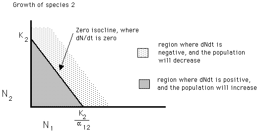
- Graph is in "species
1 and species 2 space" (see diagram axes) below
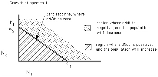
- the idea of a zero isocline is a
line that represents all of the combinations of species 1 and 2 (which
are points in 2 dimensional space) that result in one species having a
growth rate (dN/dt) of zero
- make sure you are comfortable
with this idea and also the fact that the lined region is where dN/dt
is greater than 0 (where the population of species 1 will increase
in number) and the checked region is where the growth rate is negative
- to do this look at where
K1 is and imagine that there
are no species 2 present (so you are along the x axis) and then
go beyond K1 to the right
- this is obviously where
the population must get smaller and it is also where the checked
region is!
- Now, do the same
for species 2
- Using these two expressions
as a linear prediction of where each species will have a growth rate of 0,
we can see under which conditions exclusion and coexistence are predicted.
- We must superimpose
the two graphs above, so that both isoclines appear on the same axes,
then we can judge graphically what outcome is predicted
- When one species has a zero growth
isocline greater than another at all points, that species will be
able to grow under some conditions where the other decreases.
- Here, region B is where the population
of Species 1 can get larger and Species 2 will get smaller
- This growth and shrinkage will continue
until Species 2 hits the x axis (where its population size is 0 and
it has gone extinct)
- Species 1 will then grow to its K1,
which is its carrying capacity, and it is the winner
- The situation is reversed
if the isocline of Species 2 is farther from the origin than Species
1 (Species 2 is the winner when it hits K2)
- and are equilibrium points, as the
population sizes will not change unless something disturbs the system
- Now, lets look at the
situation where both are present and the zero growth isoclines do intersect.
- Depending on the
relative sizes of K1, K2, a1 and a21, either stable or unstable equilibria
are predicted
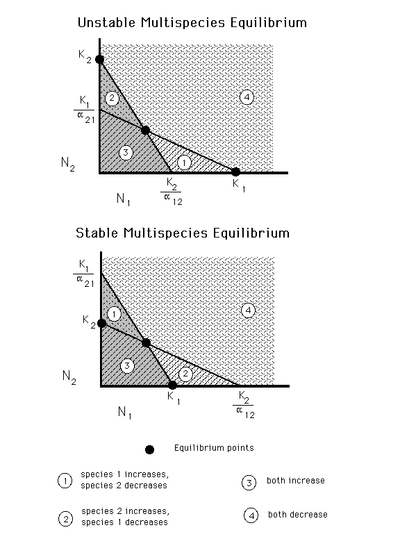
- the important areas
here are 1 and 2
- to understand why the top is unstable,
go to these areas and predict how the populations will change
- to do this, look at the zero
isoclines to decide what will happen to each species
- you will get a similar situation
as when the lines don't intersect (one species will go extinct
and the other will go to its carrying capacity
- thus, when the equilibrium
is unstable, one species wins and the other loses when the system
is displaced from the equilibrium point represented by the intersection
of the zero isoclines
- in the lower diagram, the regions
1 and 2 are reversed (you can see why if you look at where they are
with respect to the zero isoclines)
- now if you predict where
each species will go, you see that you will head back towards
the intersection of the zero isoclines
- thus, any disturbance will
just result in return to the equilibrium point with both species
present (unless the disturbance is so severe that one species
is eliminated, which is a point from which it can not recover.
Competitive
Exclusion Principle
- When two species that
require the same set of resources and one is better able to gain access to
the scarce resource or resources, then one species will exclude the other
from that locality
- Related to the idea
of a niche, a "space" describing
all of the needs and abilities of a species
- Restatement of the
competitive exclusion principle is that no two species can occupy the
same niche
- some see a niche
as a geometric space with each important abiotic factor or resource as
an axis (so this space has many more dimensions than the three normal
space has)
- Called a principle,
but it must be proven in each case, and so it is not a principle but a hypothesis
- Competitive Exclusion
Principle restated in terms of the niche is: no two species can occupy
the same niche. Defining the principle this way
brings up an observation and a question:
- Competition is the
mechanism of exclusion, so the only niche factors that influence exclusion
are those that have something to do with the limiting resource or resources
- Just how similar
can two niches be before one of the species is excluded? Look below
under the "Coexistence and Competition" section!
- Niches can be altered
by presence of competitors or predators that reduce the total "space"
occupied by a species
- fundamental
niche - maximum niche when no competitors, predators, parasites,
etc. present
- realized
niche - actual space occupied by the species when other species
are present
Factors
that Influence Competition
Temporal
Heterogeneity
- Changes in a habitat over time
may shift the competitive advantage from one competitor to another.
- Seasonal changes in temperature
or rainfall can favor different species
- Changes in habitat due
to age of habitat can alter competitive relationships
- Tribolium
- Two species
of beetle living in stored grain and flour (important pest species)
- Almost
always, one species ousts the other, but not always the same
species wins
- mechanism
of competition is predation of eggs and pupae by larvae
and adult beetles
- Some
see this not as competition, rather as mutual predation,
but the outcome is the same
- Sporozoan
infection first altered the outcome (T. confusum more
resistant and won)
- Abiotic
conditions affected outcome
- T.
confusum won when flour dry, T. castaneum when
wet
- T.
castaneum wins when grain is fresh, T. confusum
when grain has dried .
- Among my yeast, some
yeast species are excluded from the rot by competitors under the
conditions found in recently dead tissue but are competitive dominants
when the tissue ages.
- Disturbance from unusual
events (storms, droughts, early freezes, HUMAN ACTIVITY) can alter competitive
outcomes.
Spatial
Heterogeneity
- Gradients
(Clines) can change competitive
outcomes.
- One species dominates one
end of the gradient, the other species dominates the other end, and
coexistence occurs in between.
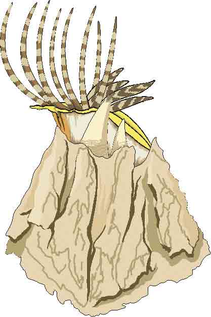
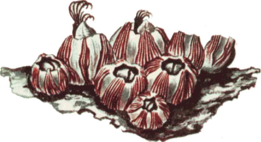
- Barnacles in the Rocky
Intertidal - Connell
- The tidal cycle
sets up a gradient along the rocky shoreline, with the lower rocks covered
by the tide for longer than the upper rocks
- the rocks
offer a hard substrate to which animals and algae can attach and
feed on (or absorb nutrients from) the water that flows over them
(sandy shorelines lack the opportunity for attachment)
- Barnacles
and mussels are both filter-feeding animals that benefit from the
water flow
- Chthalamus
upper limit set by desiccation, lower limit by Balanus
- Remove Balanus and Chthalamus grows
- Remove Chthalamus and Balanus does
not invade
- Balanus
upper limit set by desiccation, lower by starfish predation
- Remove predators and Balanus invades
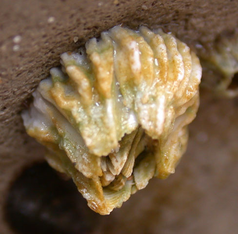
- To refresh your memory about barnacles,
remember that they are crustaceans that are sedentary as adults.
They lie on their backs on a rock and build a calcareous shell around
themselves (some have stalks that attach them to the rocks). When
they feed, they extend their legs and use them as a net to filter food
particles from the water. I thank Arthur's
Clipart Site for the following images.
Coexistence
and Competition - Niche relationships
Resource
Partitioning
first discussed in "Homage
to Santa Rosalia or why are there so many kinds of animals?" Hutchinson,
1959
- Asked an important
question - if competition has the power to exclude all but the best competitors,
why then are so many environments full of similar species
- looked at a kind
of bug found in ponds and found that more than one species of these
bugs, which all look alike and feed in the same manner, occurred in
the same ponds
- question was why did
not the best competitor force the other species out?
- Concluded that
species were Resource Partitioning
- Species were monopolizing a portion of the resource but not the entire
resource
- In the case of
the ponds, the species of bugs would not coexist if their feeding apparatus
was too similar (they could not exceed a maximum similarity - called
the Limiting Similarity)
- Similarity
can be expressed as a ratio between the size of two species (or
the size of some body part important in dealing with the limiting
resource)
- Hutchinson measured this ratio
as somewhere around 1:1.28 for his bugs in the ponds near Santa
Rosalia and he called this ratio the Limiting
Similarity
- many went out and found the ratio
and concluded that competition was the cause
- Limiting similarity
has bee criticized for non-experimental nature of findings and for
the fact that the same ratio often occurs where no competition exists
- These ideas about
competition all assume that there is a limiting resource (usually 1, but
two or more have been considered)
- many have modeled
resources as resource niche axes:
- Resource
Axis -- a line representing change in a resource, such
as size, or sugar concentration, or concentration of toxins
- Species
Utilization Curve -- the degree to which a species can
utilize a resource at some point on the resource axis
- Different species
can be represented as humps along the axis
- humps (usually bell shaped, but not
necessarily so) give each species range of resources sizes utilized
and its optimum resource utilization point
- Niche
Overlap -
the portion of the resource axis (or axes) shared by competing
species
- Ideally, if limiting similarity is
correct, the overlap between species resources will not be larger
than the limiting similarity ratio
- Species
Packing -- when all of the species on a resource axis are
spaced so that each shows maximal overlap allowing coexistence (therefore,
no additional species can be added without causing more overlap than
limiting similarity would allow) the resource axis is called "packed"
Measuring
Niche Overlap
- What happens when
the niche dimension is not a continuous variable, so that an axis can't
be used to describe it?
- this situation might
describe a resource that is uniform (like suitable space) but occurs as
patches separated by unusable space
- here we can use a
different measure of niche and a different measure of overlap
- Niche breadth
- Niche breadth is the degree
to which a species utilizes all available patches or resources
- there are many ways to measure
this, but all are related to the simplest given below (Levin's niche
breadth)
- here the symbols are
- S = number of resources
or patches of resource
- pi = proportion
of a species utilizing the ith resource or patch
- will range from 1.0 when the
species is equally distributed across each resource or patch or 1/S when
all members of a species are found on one patch or resource
- the pi's are often measured
as the proportion of different food types in the guts of the species of
interest
- Overlap between the breadth
of two species (here designated species j and species k) may be as Proportional
Similarity (between the two species)
here, pij and Pik
are the proportions of the least-abundant species found on the
ith patch or resource
As a rule of thumb, a PS of
over 70% is considered to indicate active competition between the species,
and lower values allow coexistence of the competitors
Competition
and Evolution
Competition is an important influence
on the success of organisms and so, competition will affect the fitness of
organisms and characteristics of organisms that are important in competition
will be subject to natural selection. Below we consider two aspects
of this relationship.
- Character
displacement
- Best evidence for
limiting similarity
- When species are
allopatric (look at lecture on modes
of speciation). their utilization patterns (as reflected by their size
or the size of their mouth parts) overlap (ratio is below 1:1.1 or so)
- When they are sympatric,
the overlap is reduced (indicated by larger ratios of the magnitude from
1.3 and 2) due to Character Displacement
- so character displacement is the
evidence of past competition forcing species that were too similar
to become more dissimilar in order to coexist
- Has been shown for
Darwin's finches in the Galapagos islands
- r
and K selection
- Remember that K
selected species are thought to experience competition but r selected
species simply move on to new, unexploited resource rather than compete
for resource in a crowded patch
- r-selected
species are species that experience local patch extinction
and live by colonizing new patches
- they rarely
experience carrying capacity, and often grow near to the maximal rate
(~r when N is low for the logistic)
- K-selected
species occupy more long-lived patches, which can become saturated
and so they experience carrying capacity (K)
- When one characterizes
species by this dichotomy, then "suites" of characters are associated
with each type of selection
| Character |
r-selected species |
K-selected species |
| Mortality |
density-independent |
density-dependent |
| Survivorship |
type III |
types I, II |
| Population Size |
variable |
constant |
| Competition |
minor |
keen |
| Life expectancy |
short |
long |
| Fecundity |
high |
low |
| First reproduction |
early |
late |
| Type of reproduction |
semelparous |
iteroparous |
| Body size |
small |
large |
Cited
Literature
Connell, J. H. 1961a.
Effects of competition, predation by Thais lapillus and other
factors on natural populations of the barnacle Balanus balanoides.
Ecological Monographs 31:61-104
Connell, J. H. 1961b.
The influence of interspecific competition and other factors on the distribution
of the barnacle Chthalamus stellatus. Ecology 42:710-723.
Hutchinson, G. E. (1959). "Homage to Santa
Rosalia or why are there so many kinds of animals?" American Naturalist
93(870): 145-159.
Terms
Mutualism, Commensalism, Competition, Allelopathy,
Herbivory, Predation, Parasitism, Amensalism, symbiosis, Interspecific Competition,
Lotka-Volterra Model, Trivial equilibrium, Stable Equilibrium,
Unstable Equilibrium, Zero-Growth Isocline, niche, Competitive Exclusion Principle,
Fundamental Niche, Realized Niche, Gradient
(Cline), Resource Partitioning, Limiting
Similarity, Resource Axis, Species Utilization Curve, Niche Overlap, Species
Packing, Niche breadth, Proportional Similarity,
Character displacement
Last updated February 17, 2007