BIOL 4120

Principles of Ecology

Phil Ganter

320 Harned Hall

963-5782

Buried under the sand at the bottom of the pit above, an antlion (a neuropteran larva) sits and waits for in small animals to tumble down the walls of the pit and into the jaws that suck the prey's body fluids.  More on doodlebugs (another name) here or here

Lecture 14 Predation/Herbivory

Email me

Back to:

Overview - Link to Course Objectives

Predation and Herbivory

An interaction between two species in which one is harmed and the other helped

Several flavors of interaction fall under the above rubric:

  • Herbivory -- plant eaters, algae not usually considered but included
  • Carnivory -- meat eaters (other carnivores or herbivores)
  • Cannibalism - eating one's own species - a specialized form of predation
  • Parasitoids -- usually insects that lay their eggs on other insects as hosts. The larvae complete development on the host, usually killing the host as a result
  • Parasitism -- feeding on another organism's parts without killing the organism (a note: parasitism is very widespread and includes all kingdoms as both parasite and host)

The chart below can be helpful in separating the types (adapted from text)


Lethality to host

Contact between organisms

Low

High

Close and Long-term

Parasites

Parasitoids

Brief

Herbivores

Predators

Both predation and herbivory are +.- species interactions in which one species benefits from the contact and one is harmed.

  • Predation is a form of carnivory in which food items (prey) are searched for (or waited for), caught and killed.
    • Predators tend to be much larger than prey to minimize the risk to the predator (predators do not give the prey a "fighting chance" and there is very little "struggle" in the struggle for life)
  • Parasitoids are insect predators differ from the standard model of predation.
    • The adult searches for and captures the prey.  
    • Eggs are then laid on the prey.
    • The larvae hatch and eat the prey, pupate, and emerge as adults to search for prey for their offspring.
  • Herbivory is a bit the same as and a bit different from predation.
    • It involves plants.
    • Herbivores may be much larger (cattle eating grass) or much smaller (caterpillars eating leaves on a tree) than their food items.
    • Herbivores must also search for food items.
    • The food items are usually not killed but are damaged by the herbivore.
    • If the herbivore eats the seeds, then the plants are killed and some large herbivores do kill the plants they attack (elephants often knock down trees to get to the leaves, cattle and sheep sometimes pull out the plant by its roots).
    • Predator-prey interactions are usually of short duration.
    • Some herbivores spend the rest of their lives on the plant once it is found (sometimes multiple generations).

A better way to look at this might be to divide herbivores into those that are like predators and those that are like parasites

  • Predator-like herbivores are larger than their food items, the encounter between herbivore and plant is of short duration compared to length of herbivore's life, and the encounter may kill the plant.
    • Many vertebrate herbivores might be in this group,
  • Parasite-like herbivores are smaller than their food items, the herbivore-plant encounter lasts for a long time, and the plant is usually not killed.
    • Many insect herbivores are in this category.

Modeling Predation

We will use an approach that builds on the logistic that we have worked with previously

First, we assume that the prey population will grow exponentially except that the predator is there to eat some of the prey

  • The number of prey consumed depends on the number of prey present, the number of predators present, and a fudge term called a, the "searching efficiency", which can not be determined theoretically but must be measured for each combination of predator and prey.

If we set N as the number of prey, C as the number of predators, and use other, familiar terms, then the rate of change of prey is:

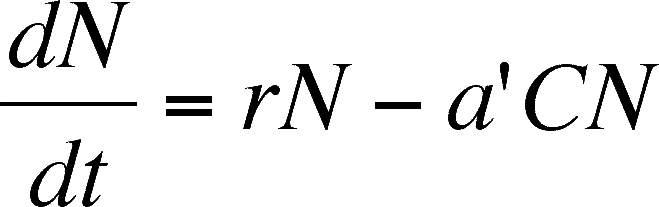
Read this equation as: The rate of change in the number of prey present (dN/dt) is a function of the birth of new prey (rN) minus the death of others due to predation (a'CN). The death rate is assumed to depend on the number of prey, the number of predators (C) and the fudge factor (a').

The rate of change in the predator population is:

Read this as: The change in the number of predators present is a function of the birth of new predators minus the death of others due to some constant mortality rate (old age? mishap? parasitism?). The birth rate is assumed to depend on the number of prey (the resource the predator uses to make new offspring), the number of predators (more predators, more predator offspring), a' (the ability to catch prey), and a second fudge factor called f, which is the efficiency with which predators turn their food (prey) into offspring.

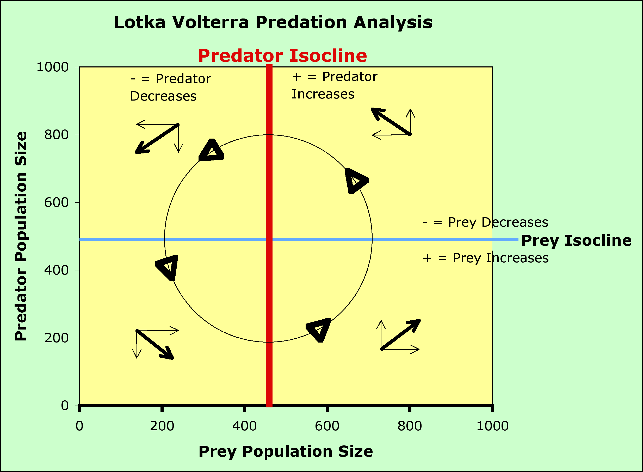
Taking the same tack as before, we solve these equations for conditions where no growth is taking place (hence some sort of equilibrium) by substituting 0 for dN/dt and for dC/dt:

Prey zero isocline:

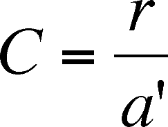
So, prey numbers do not grow when the number of predators is equal to the ratio of the prey's intrinsic rate of increase (a property of the prey) and a', the searching efficiency of the prey-predator combination (the graph of this is a straight line parallel to the prey axis - usually the x axis). When the number of predators is below this line, the prey increase, when the predator number is above the line, the prey decrease.

Predator zero isocline

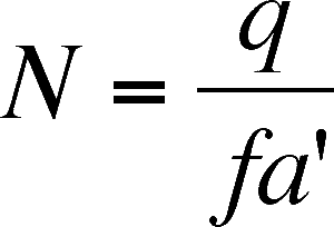
So, predator numbers do not grow when the number of prey is equal to the ratio of the predator's intrinsic death rate (a property of the predator) and the product of f and a', (this is also a straight line but is parallel to the predator axis, not the prey axis - usually the y axis). When the number of prey is to the left of this line, the predators decrease (not enough prey per predator). When the number of prey is to the right of this line, there are sufficient prey per predator and the number of predators increases.

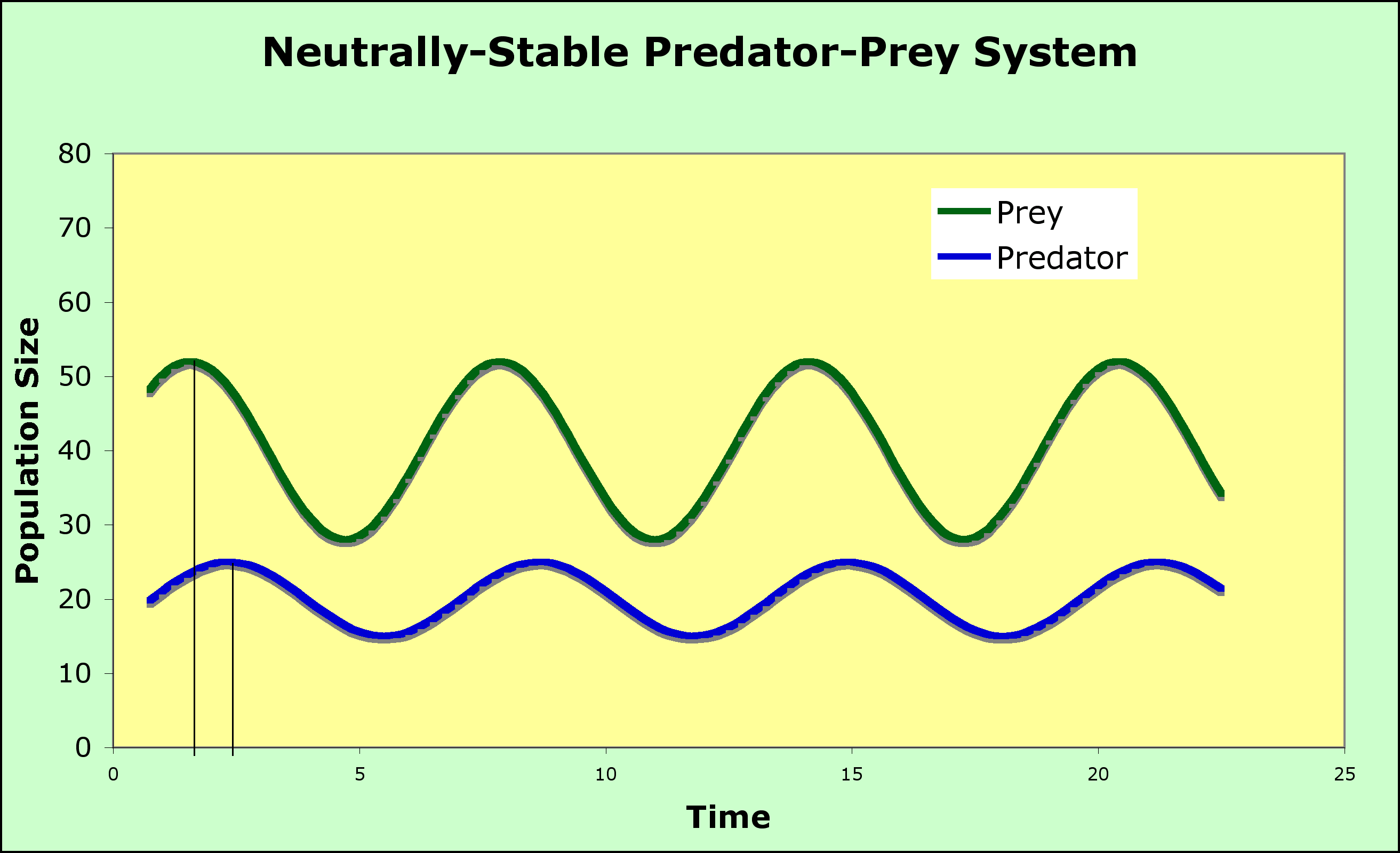
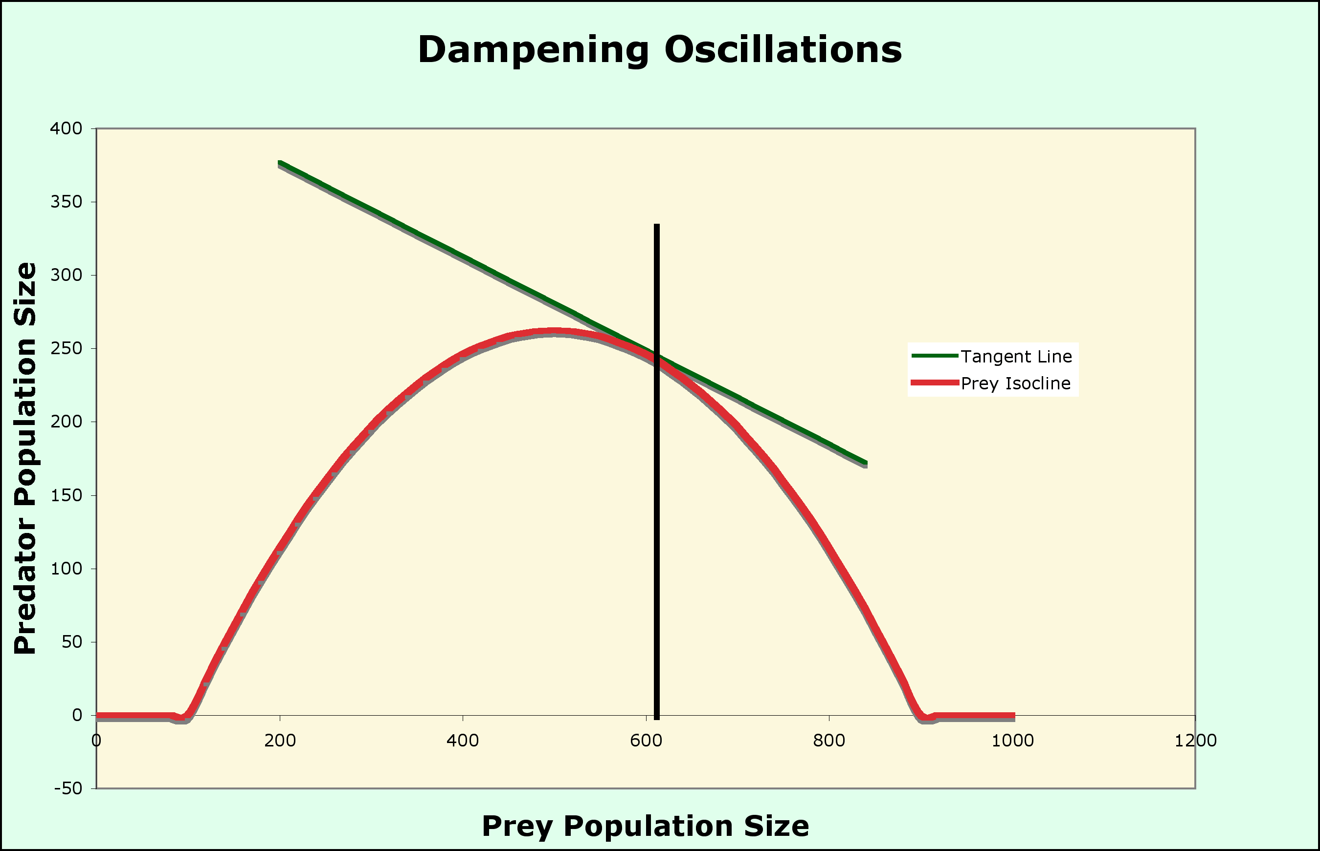
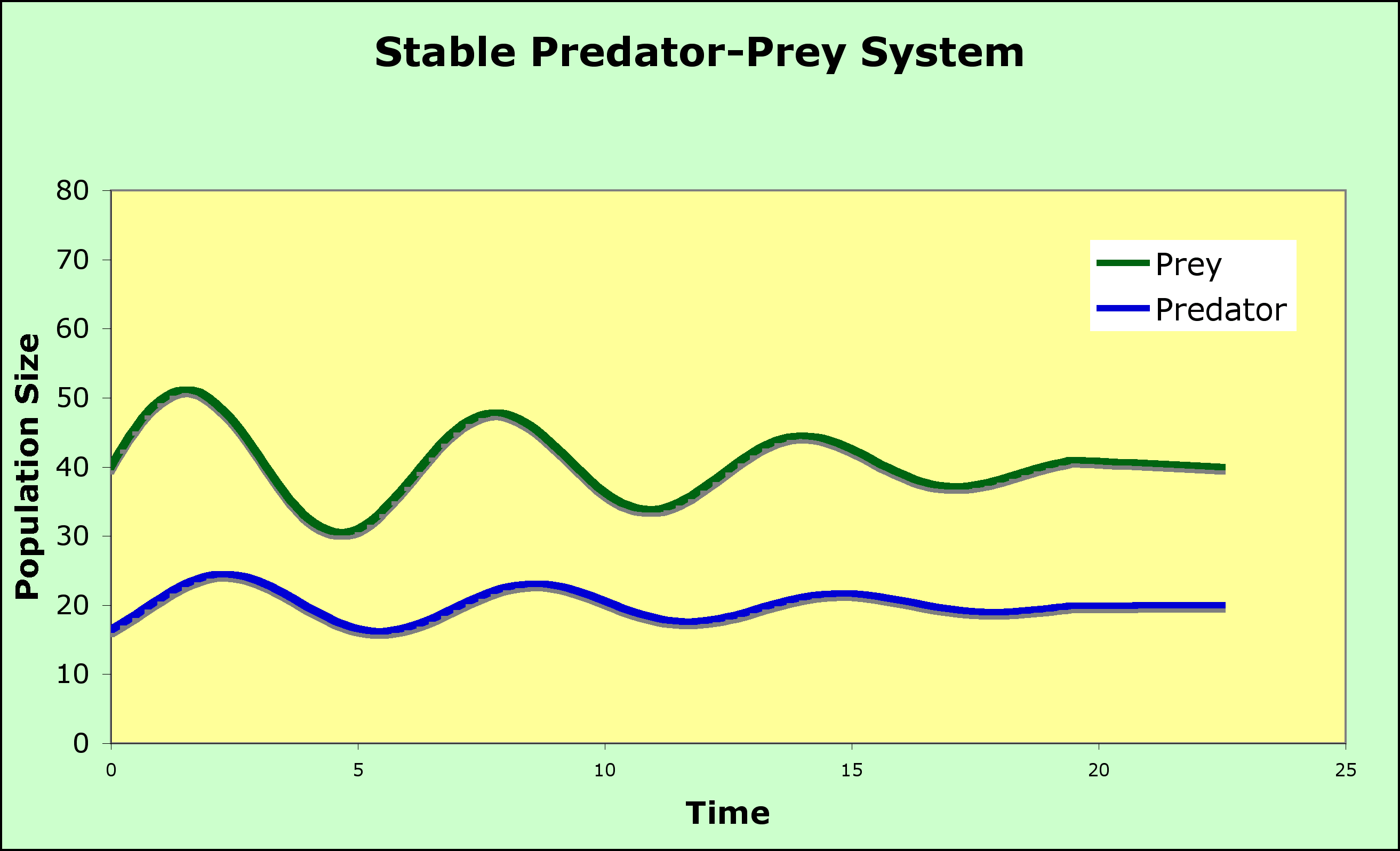
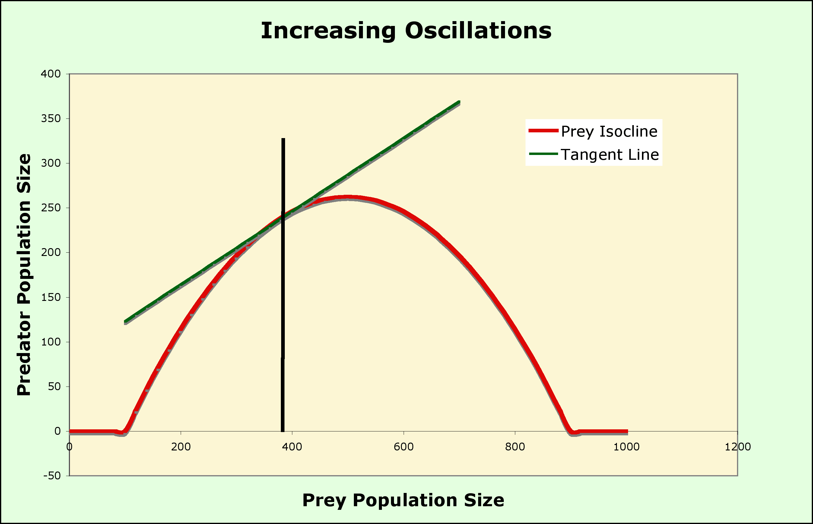
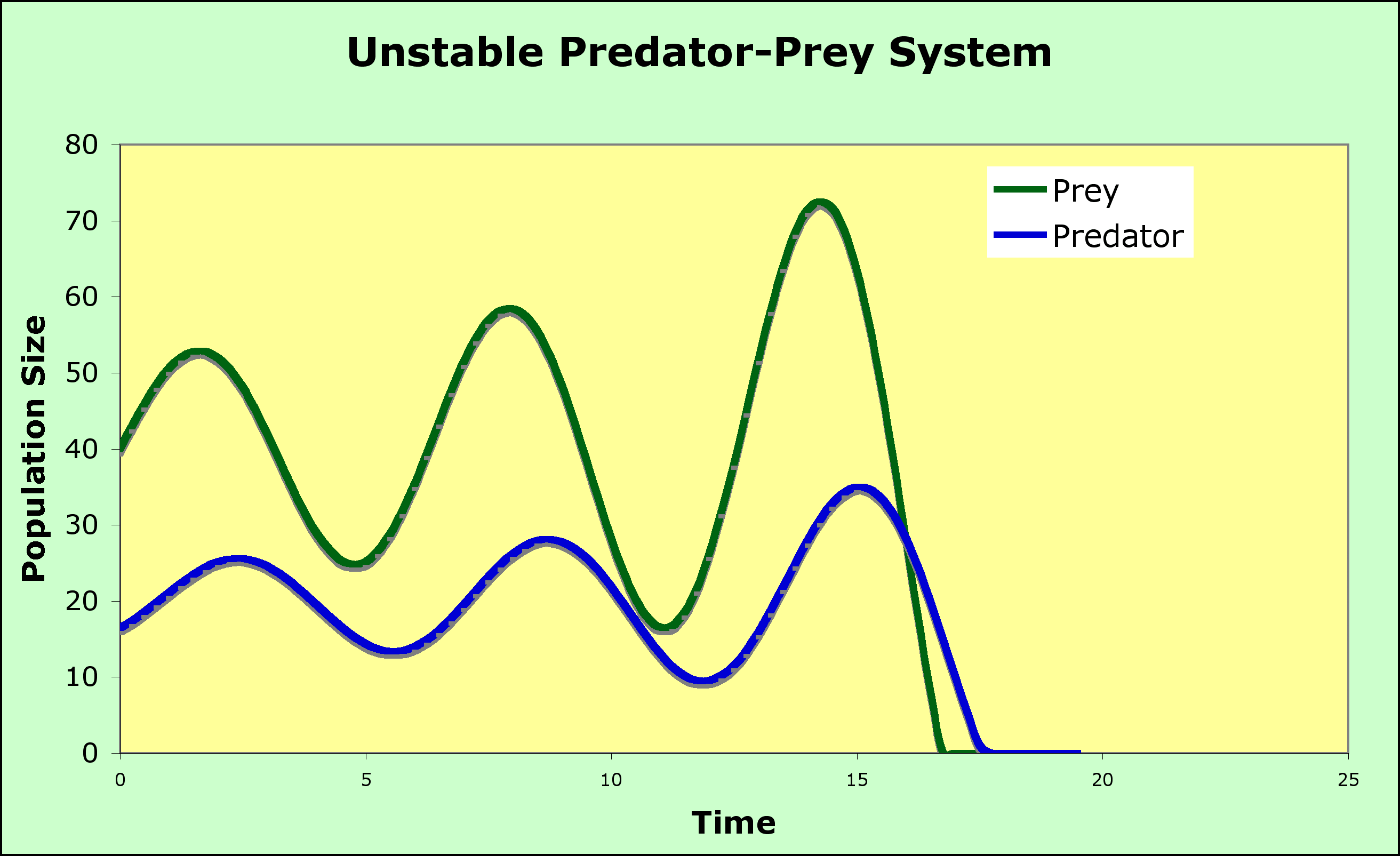
This situation leads to an Equilibrium (where the isoclines cross).

  • The blue and red lines are the zero growth isoclines
    • Look at the + and - regions for predator and prey on the graph - be sure you understand why above the blue line the prey population decreases and why the predator population decreases to the left of the red line.
    • Look at the vector addition arrows - be sure you can explain the direction of each set of arrows
    • Look at the circle and the arrowheads on the circle - be sure you can explain why the arrow heads indicate counterclockwise motion.
  • Notice that there are no other equilibrium points on the axes except for 0,0 (the origin) where neither are present
    • With no prey present, the predators decline to 0
    • With no predators present, the prey population takes off to infinity (exponential growth, as we mentioned at the beginning of the modeling effort in this chapter)
  • The second equilibrium point is where the isoclines intersect
  • These equations are neither stable nor unstable (this condition is called neutrally stable), as the system will oscillate in what is called a predator-prey cycle - see graph below
    1. prey increase until there is enough for predators to start to increase
    2. predators increase until they eat enough prey to cause a decline in the prey population
    3. prey start to decline in number until predators can't find enough to eat and the predator population declines
    4. prey begin to increase, and we are back at step 1
  • Some evidence for these under special circumstances
    • Lynx and hare

The predictions of the model can be modified by changing the shape of the isoclines to include:

  • Prey self-limitation
    • this is done my making the prey zero isocline (the horizontal line) curve down as the number of prey increase so that, even if there are no predators present, the prey will decline past the point where the isocline crosses the x axis
    • the crossing point is K, the carrying capacity of the environment
  • Interference between predators when they are numerous and prey are scarce
    • this is done by bending the predator zero isocline, the vertical line (q/fa'), to the right
    • think about what this means
    • the level of prey that results in a decline in predators now increases as the number of predators increases, which makes sense
  • Under these situations, stable coexistence is possible as the cycles diminish in their amplitude as time goes on.

A Graphical model of Predation

Now that you are used to a graphical analysis of species interactions, a completely graphical analysis of predation first proposed by Michael Rosenzweig and Robert MacArthur can be used to stabilize the model above


  • note that the lines are still ZERO ISOCLINES, where the predator or prey populations are neither growing larger nor decreasing
  • to analyze the graphs, make sure you
    • 1. understand why the graphs are the shape they are
    • 2. understand what happens when the populations are not on the lines (in which areas the predator and prey populations are increasing and decreasing)
  • The left side of the humped prey zero isocline (where it hits the X-axis near 0) is the smallest population of prey that can successfully find mates.  It can be as small as 1 prey.
  • The upper bound, where the prey isocline crosses the x-axis on the right side, is K, the prey's carrying capacity.
    • The prey isocline is humped because, at low prey population size, it takes more and more predators to reduce prey growth to zero as the number of prey increases. So, the prey zero isocline first goes up. As the prey population gets closer to its carrying capacity (K), the number of predators needed to check prey population growth becomes fewer and fewer, as each prey becomes more and more food limited.  Food limitation means lower reproductive success, so fewer predators can keep the prey population in check. Thus, the prey isocline goes down as it approaches K.  First up and then down makes the hump.
  • The predator isocline has not been changed in the above graph.  Subsequent alterations to the model might allow the predator isocline to have a slope (the slope is undefined in the above graph) and might include a predator carrying capacity.
  • Notice that all of the graphs have an intersection between the two isoclines, so there is an equilibrium possible that allows both predator and prey to coexist in the system. The question: Is that equilibrium stable, neutral, or unstable?
    • Stability analysis of this, the simplest, version of the Rosenzweig-MacArthur model depends on the slope of the prey zero isocline when it intersects the predator zero isocline (NOTE - the slope a curve at any point is the same as the slope of a straight line tangent to the curve at that point - look above to see the tangent line drawn in in green).
      • The neutrally stable equilibrium occurs in the R-McA model when the prey and predator isoclines are at right angles. The prey zero isocline is a curve, so it is not the curve that is at a right angle (that makes no sense), but the right angle is formed by the line tangent to the curve at the point of intersection with the prey zero isocline and the predator zero isocline.
      • The predator isocline is a vertical line, so the tangent line is at a right angle to it when the tangent line is horizontal, which happens at the very peak of the prey zero isocline curve, the top of the hump

    • When the slope of the prey zero isocline is less than 1, the oscillations are dampened until there is no predator-prey oscillation in the system, which is a stable equilibrium.  The slope is less-than-1 at any point on the curve to the right of the top of the hump.

    • When the slope of the prey isocline is greater than 1, the oscillations increase until one of the species population sizes, predator or prey, falls to 0. The slope is greater-than-1 at anypoint on the curve to the left of the top of the hump.

    • If it is the predator that is lost, the prey goes to its K.  If it is the prey that is lost, the predator soon follows. This is an unstable equilibrium.

Two variations

  • Refugia for the prey make it impossible for the predators to drive the prey from the system There is a portion of the prey population that can't be eaten and these can always repopulate the portion that does get eaten.
  • Paradox of Enrichment
    • the prey isocline is extended by a change in K (that is a result of the enrichment of the prey's environment so that the prey's carrying capacity is increased)
    • this changes the shape of the curve or moves it. If this change in shape means that the intersection of predator and prey isoclines are switched from a point at which the prey isocline's slope is negative to one where it is positive (look at the graph), then the stability of the system is changed from a stable to an unstable equilibrium, where either predator or both predator and prey are lost from the system

    The paradox is that, by enriching the environment, you destabilize the system! Not all good acts have the intended outcome.

Optimal Foraging

Predators with more than one available prey type must decide which prey to pursue.  Optimal Foraging theory has been developed to understand the factors that govern this decision for any organism with more than one choice of food. 

  • This theory applies to any situation in which there is a choice between food of different quality (different types, large versus small items of food of the same type, high versus low quality food items of the same type). 

Optimal Foraging is based on some assumptions. 

  • The forager must make its choice based on maximizing its intake of some aspect of its food (calories, an essential nutrient, etc.). 
  • There must be a cost to each choice.  This cost can be the difficulty of "handling" the food, ingestion of a toxin found in the food, the time it takes to search for the food, the chance that searching will expose the forager to a predator, or some other cost. 

Optimal foraging is another example of a Trade-Off based on costs and benefits. 

  • Optimal forager will choose prey to maximize the benefit/cost ratio. 
  • This often means that the optimal strategy is to avoid a choice prey item if the costs are too great.

Search Strategy

How should a predator find its prey? 

  • Some predators are Sit-and-Wait Predators.  Here the search strategy involves the choice of a place in which to wait. 
  • Active, hunting predators search in a heterogeneous environment composed of patches with prey, patches without prey, and some distance between patches. 

The Marginal Value Theorem (from economics) predicts the length of time a predator should spend in a patch based on the distance between patches, the rate of prey discovery within the current patch (more elaborate versions of the model include variation among quality of patches). 

  • The best strategy is the one that will maximize the predator's total intake of some aspect of its food (total prey caught, total calories, total of an essential nutrient, etc.) over the total search time available to a predator. 

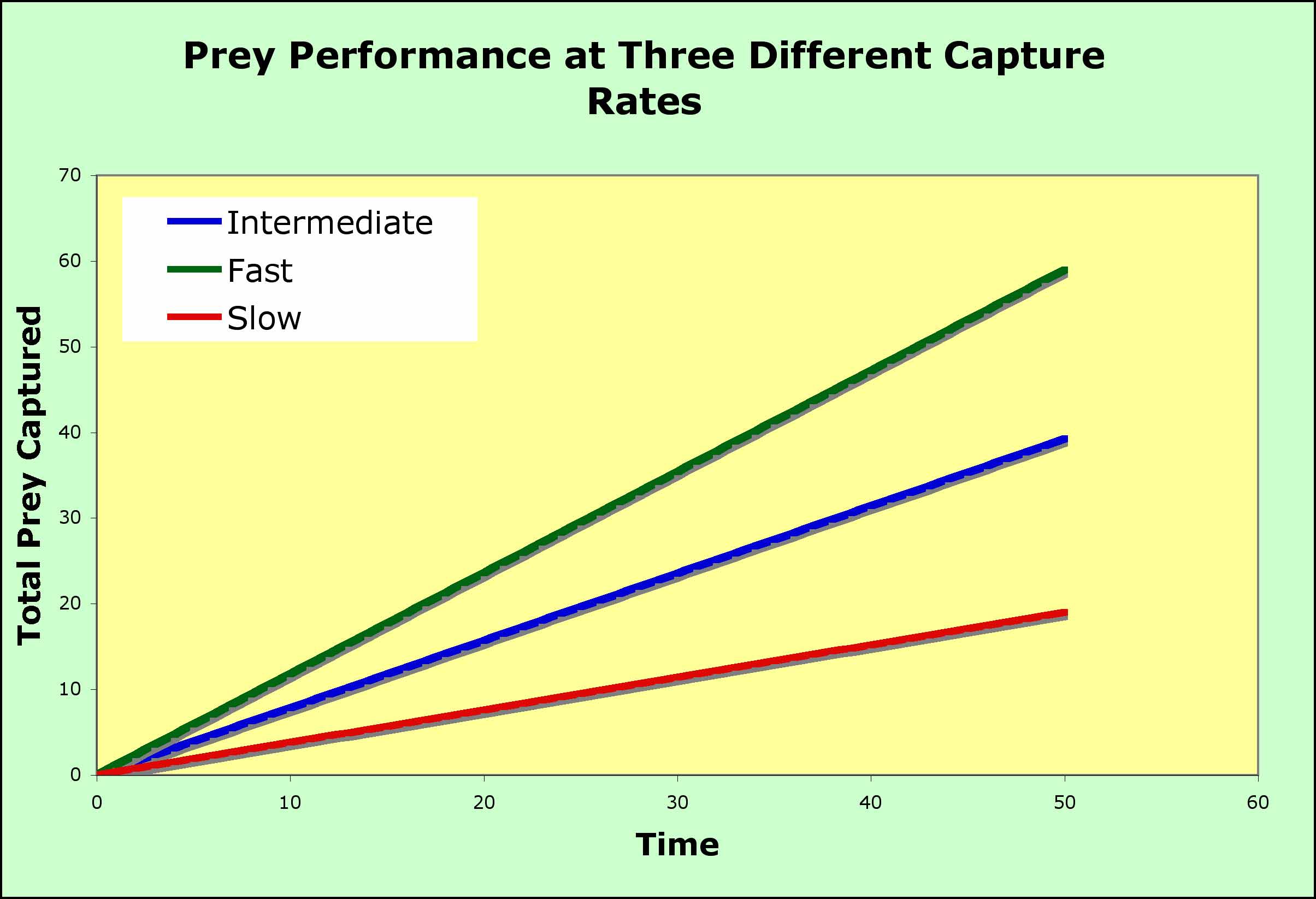
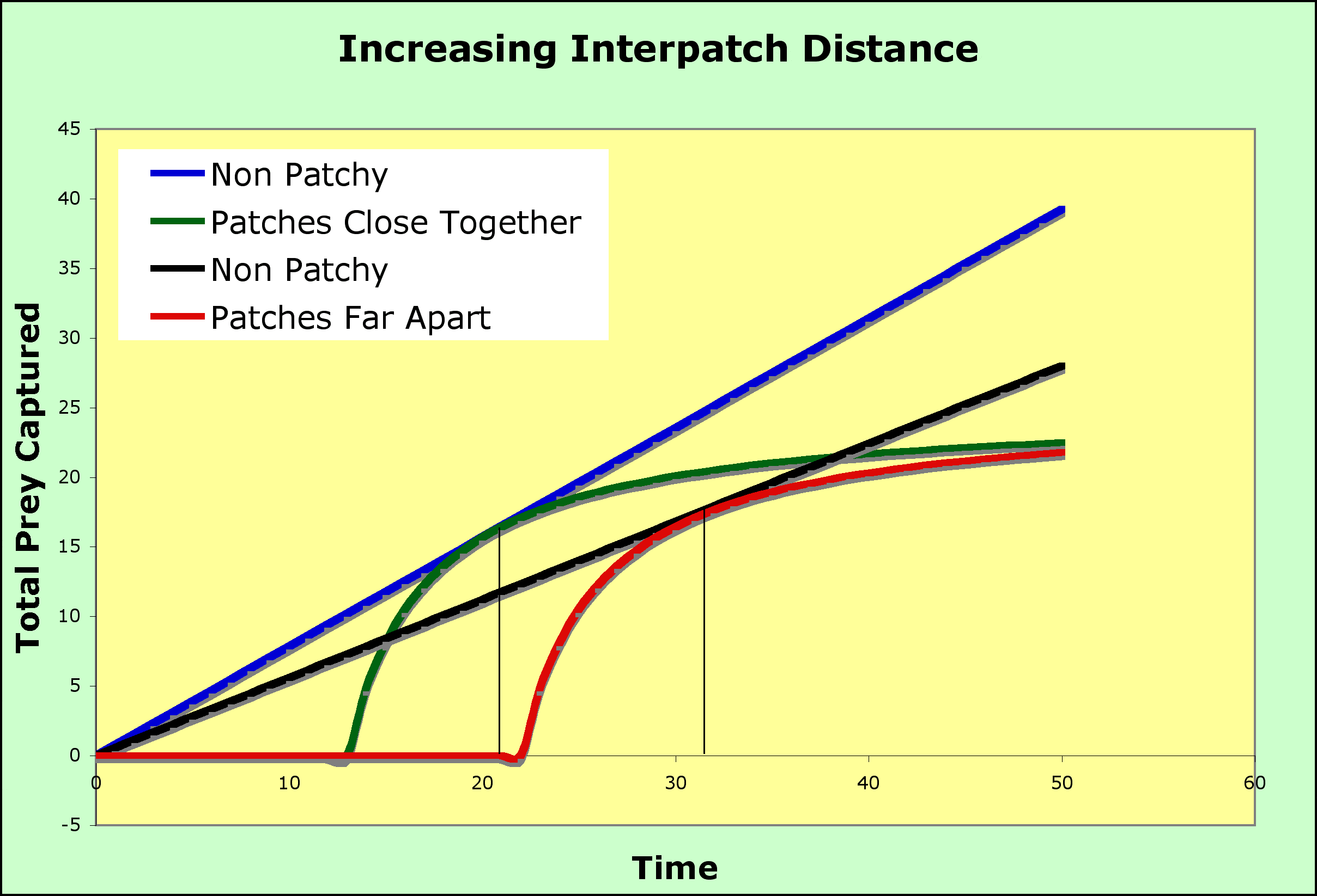
    • consider the environment without patches (the graph above), where food is distributed randomly throughout the habitat
      • the animal enters the habitat and begins to search.  food and encounters the food randomly
      • the longer the animal searches, the larger is the total catch and the increase can be predicted by a straight line
      • the slope changes with the density of the prey, so that the rate of capture can be fast or slow
    • the straight lines above represent the best that a predator can do in terms of prey capture given a particular density of prey
  • So, what happens when we introduce patchiness into the habitat so that the prey are not randomly distributed but are found in clumps?
    • The model assumes that there is a cost (in terms of time) to travel to a patch and that there will be another patch available if the current patch is abandoned, although it will cost time to find it.
      • The flat portion of the green curve on the graph below, the portion that runs along the x-axis, represents the time it takes to find a patch during which no prey are captured
    • After the predator arrives on a patch, it will begin to eat prey and the total intake will begin to rise. 
      • This rise is the upward portion of the green curve. Note that it rises very fast, which is reasonable because the predator is in a patch with prey close at hand
    • At some point, the predator will begin to deplete the patch and the intake will slow. 
      • The slowing intake causes the total intake curve (total intake plotted versus time spent to reach the patch plus time spent in the patch) to "plateau," to flatten out, and when no new prey items can be found, the total stays flat as time goes on: no new prey, no increase in the total.  Surely, it is time to leave. 
  • When should the predator leave the patch?  before the plateau? when the plateau is reached?  some time after the plateau is reached? 

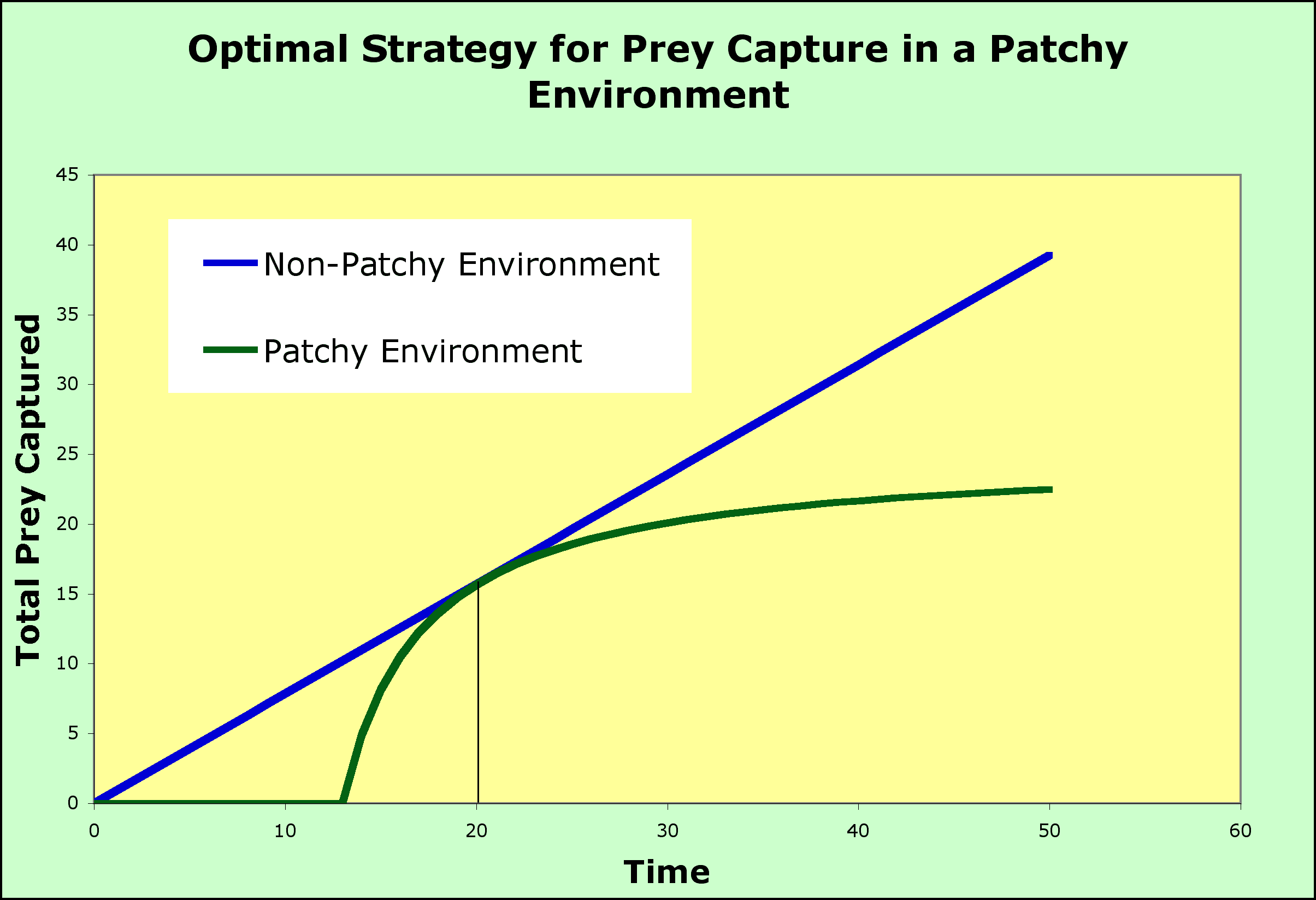
  • The marginal value theorem says to leave before the plateau is reached.  The predator should  not wait for the plateau but should leave when the rate of return (intake of prey per unit time) is at its maximum.
    • The maximum will be where the total intake in the patchy environment (the green cruve) equals the total from a non-patchy environment (the blue line) - at that point the predtor has done as well as it possibly could have but if it persists in the patch, the falling rate of prey capture means it will fall behind in total prey caught (if it leaves before the intersection point, it will not have acheived the maximum).
  • By doing this, the patch is abandoned and the search for another patch begins so that the total intake over the entire search time is maximized. 
    • If the predator stayed in each patch until all prey were captured, it would visit fewer patches and much of its time on the patches would be spent searching for scarce prey (prey made scarce by the predator itself).

Searching time and patch size or quality both affect the time spent in a patch.

  • As search time gets larger, the time spent in a patch will increase.  The relative benefit of leaving is reduced due to the increased time before the next patch is found.
    • In the graph above, longer search times to find a patch results in the tangent point moving to the right on the red curve where patches are far apart and the search time is longer (moved to the right compared to the tangent point on the blue curve, where patches are close together and so the search time is shorter)

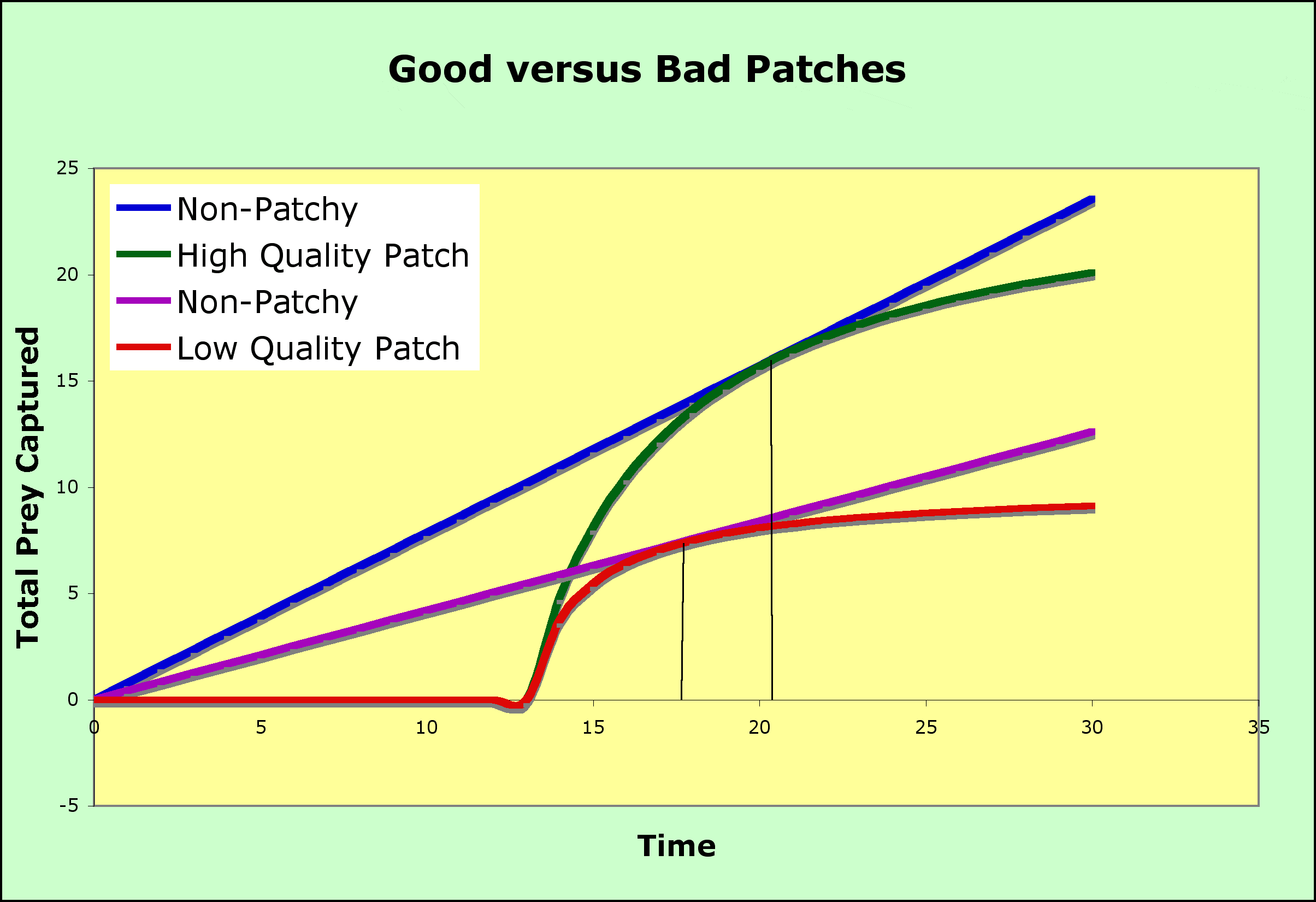
  • Low-quality patches increase the time spent in a patch compared to high-quality patches
  • for patches of higher quality, the prey captured curve goes up faster and plateaus higher (the green curve) than for low quality patches (the red curve)

Coevolution between Predator and Prey

Changes in the predator and prey due to either the necessity of catching prey or the risk of being eaten may mean that the one species changes as in response to the other - this is and example of Coevolution.

  • Coevolution can lead to an Arms-Race as the prey changes its defenses, the predator counters with a change, to which the prey then responds.
  • This means that evolution is an ever-ongoing process and that change is a necessity.  This concept has become known as the Red-Queen Hypothesis - running (evolving) as fast as you can just to stay in place.

How important is predation in nature?

  • If not important, prey will have no special adaptations for avoiding predation. No risk, then no reward for avoiding it.
  • If important, then some type of strategy for predation avoidance will be a common adaptation
    • By this criterion, predation is an evolutionary significant source of mortality, as the strategies below are widespread
    • may be more likely to see anti-predator adaptations rather than predator adaptations because of the Life-Dinner Principle
      • The selective pressure is greater for the prey, which loses its life if it is unsuccessful, than on the predator, which only loses its dinner if it fails
    • however, evolution may respond to small differences in mortality, too small to be ecologically significant
      • to decide on the ecological significance of predation, field experiments are necessary (see below)
      • The acorn barnacles above show evidence of heafy predation - at least half of the shells are empty.

Strategies for predator avoidance

Coloration:

  • Aposematic colors: Warn the predator that they (the prey) are distasteful
  • Cryptic colors: Hide the prey by blending it with its background
  • Mimetic colors: These are attempts by members of one species to resemble another species. There are several types with more than one purpose:
    • Batesian mimicry: The mimic is edible, but looks like a model species that is not palatable due to a toxin in it.
      • one could argue that this is a kind of parasitism, as the mimics are helped and, to the extent that the predators are encouraged to try an occasional prey item, the model suffers a loss of effectiveness of its poison system.
    • Mullerian mimicry: Mimics are all inedible, but are too rare for the predator to learn to avoid them, so they look like one another so that the predator thinks of all of them as a single, poisonous type of prey
      • This is done so that the phenotype to be avoided is reinforced in the mind of the predator
      • one could argue that this is a kind of mutualism among the Mullerian mimics
    • Aggressive mimicry is when predators mimic something seen as desirable by the prey so that the prey are not startled by the presence of the predator
      • Often used by sit-and-wait predators, as it makes them transparent to their prey
        • Many mantids have a flattened body and appendages that are colored like flower petals
        • sit by flowers and catch pollinators that approach the flowers for nectar

Behaviors:

  • Catalepsis - prey playing dead so that the predator ignores the prey
  • Intimidation display: an attempt to avoid predation by startling the predator long enough to get away or to convince it that the prey will be too costly to attack
    • many large eye-like patches on moth wings are felt to be useful to startle predators

Polymorphism: the presence of more than one morph in the population. Each morph has to be at a higher frequency than would be produced by mutation alone

  • can reduce predation by reducing the predator's efficiency.
    • Search images are used by predators to pick out prey from a complex visual environment
      • once a search image is formed, then the searched for morph is taken at a higher rate than its frequency in the population would predict
    • a polymorphic species can prevent a predator from forming a search image that includes all the members of the species
  • The formation of search images for polymorphic species can result in evolution of the population
    • the most common morph may suffer so much predation that it is no longer the most common morph
    • then the predator may switch its search image to the new most common morph and start reducing it
    • this kind of selection is called Apostatic Selection

Chemical defenses in prey either make the prey too toxic or smelly or too distasteful to eat

  • Toxins can poison the predator, but this often does not save the prey (only the next prey the poisoned predator never eats)
    • This strategy will only work for an individual if it is aposematically colored as the predator must know before it kills the prey that it is toxic
  • Fighting chemicals can be used to harm a predator
    • bombardier beetles explosively eject liquids to startle predators into releasing them
    • nasute termites guard the nest and spray attacking insects with disorienting chemicals
  • Some chemicals are distasteful or noxious
    • once again, aposematic coloration is needed as an advertisement of the prey's distastefulness

Masting - the production of lots of young in some years, few in others

  • Prey populations are kept low by the non-mast years, and more of the mast year young survive than would be the case if the predator population was larger due to no non-mast years
  • if masting produces great excess of propagules one year and few or none in non-mast years, the mast years may offer so many propagules that the predators eat their fill but there is little effect on reproductive success
    • if, for example, 50% of the young will die from starvation when very young with no predation, then it does not matter to the overall success if most starving young are eaten by predators.
    • periodical cicadas are believed to reproduce in their odd manner as a means of masting

Coevolution among Herbivores and Plants

Plants cannot run from herbivores but they can try to hide (see strategies below) and they can defend themselves once attacked.  This defense can take many forms and pose a problem for the herbivore.  If it does not respond to a plant's defense, it must drop that plant from its diet.  Thus, coevolution between plant and herbivore is expected.  We will discuss the forms of defense the plant might exhibit below.  As a counterpoint and to demonstrate that coevolution is occurring, we discuss herbivore responses below.  However, here it might be appropriate to ask which side is winning the war?  Probably neither, although the Red Queen hypothesis is probably functioning.  Why neither?  Two observations:  We know of no plant, no matter how well hidden or toxic, that does not have at least one herbivore adapted to feed on it.  We can also see that, although herbivores are legion and many leaves exhibit some evidence of herbivory by late summer, the natural world it full of plants and leaves.

Plant Defenses

Secondary Chemicals - those that are synthesized by specialized pathways in plant cells, not part of general plant cell metabolism

  • Some believe that they are synthesized as anti-herbivore toxins
  • Some believe that these molecules are waste products from plant metabolism and that they remain in the plant because plants are not motile, like animals, and it is safer to store the chemicals in the cells than to excrete them
    • Anti-herbivore activity is, in this hypothesis, an unintended, but useful, outcome for a molecule that would have to be there in any case
  • Contraindications that secondary chemicals are waste products
    • Waste molecules should not be costly to produce in terms of energy
    • Secondary chemicals often are costly
    • Level of herbivory often positively correlated with level of defense (more secondary chemicals produced where herbivore damage is greatest
    • Some secondary chemicals are induced
    • More secondary chemicals are allocated to valuable tissues (leaves or storage areas) than to other areas
    • Fruit often cleared of secondary chemicals or their levels reduced just prior to ripening
      • Why store waste in a place it can't stay unless it has some function there

    Two general types of secondary chemicals (based on their effect on the herbivores, not on the structure of the chemicals)

Quantitative defense

  • Chemicals build up their toxic effect, so that they often deter the herbivore or slow its growth rather than outright poison it
  • These are often a large proportion of the dry weight of living plant tissue (non-woody tissue)
    • Example: Tannins
      • Polyphenolic compounds
      • Hydrolysable tannins (can be attacked enzymatically)
        • Bind to and inactivate proteins in gut of herbivore (this is why we use them to tan hides into leather, as the binding makes the proteins tough and indigestible)
        • Interfere with digestion, can slow growth or kill
      • Condensed tannins
        • Bind to cell walls of plants and make the cell walls indigestible by fungi and bacteria

Qualitative defenses

  • Toxic in small doses
  • Usually present in low concentrations
  • Examples: Cardiac glycosides in milkweed, Alkaloids in cacti,
  • Some link the choice of secondary chemical type to type of plant
    • Apparent plants (K-selected, long-lived, large plants) tend to have quantitative defense (tannins in oaks) because their herbivores can build up over many generations on one plant
    • Unapparent plants (r-selected, weedy plants) tend to have qualitative defenses
  • Problem is that we do not often know what is an apparent versus an unapparent plant, so it is difficult to decide if this generalization is reasonable

Mechanical defenses

  • Hairs on leaves, spines on stems, thorns on stems
  • Hairs on leaves are to protect from small insects such as leave miners or those  that eat pits into leaves
  • Spines (modified leaves), prickles (sharp extensions of a plant's epidermis) and thorns (modified plant stems) are protection against larger herbivores
  • Silica bodies in leaves and stems, Calcium deposits in stems, and Lignified Collenchyma along vascular bundles
    • Grind down teeth of vertebrates and invertebrates
    • insect adults will never molt again and when their mandibles grind down enough, they starve

Failure to attract

  • Missing chemical odor or visual color cue used by herbivore to find its food
  • This can be loss of a protein from the cell membrane or cell wall of a microbe that makes it impossible for another microbe or a virus to detect its presence

Reproductive inhibition

  • Production of a hormone-mimic by plant that interferes with insect development
  • Strategy now used by many man-made herbicides
  • We do not know the long-term effect of saturating some environments with hormone-mimics

Anti-herbivore mutualisms

  • Ant - Bull Thorn Acacia
  • Ants live in bases of unusual thorns and eat Beltsian bodies
  • Ants remove other insects from the tree and even attack large herbivores (or humans)

Below-ground storage

  • Many plants survive intense grazing because much of photosynthate produced is stored below ground
  • plants with significant below-ground storage are adapted to grazing by large herbivores.
    • grasses have extensive root systems
    • many herbaceous plants  have thicken roots or separate tubers for root storage (beet, potato, carrot)

Induced Defense versus Constitutive defense

  • Constitutive defenses are produced whether or not plants are attacked by herbivores
    • Constitutive defenses are valuable if the herbivore attack might be fatal
    • induced defenses are only good if the plant survives the initial attack
  • Induced defenses are produced only after attack by herbivores or are  produced in greater amount after attack by herbivore
    • Many secondary chemicals are induced
    • Reduction of quality of leaves as food can be induces (removal of valuable materials or storage of minerals)
    • Increase in mechanical defense for leaves and stems grown after herbivore attack

Herbivore response

  • Arms race between plant and herbivore
  • Herbivores may attack plants only before defense are completely developed or before they are induced
  • Specialist herbivores have often completely adapted to presence of defense
    • Some actually need the defensive chemical for their own defense
      • Monarch butterfly protected from bird predation by presence of cardiac glycosides
      • cardiac glycosides present because the are eaten by larvae and the chemicals persist throughout pupal stage of development
  • Detoxification
    • Oxidation - mixed-function oxidases alter chemical structure through addition of oxygen
    • Reduction - addition of electrons used to modify or split apart toxins
    • Hydrolysis - splitting apart toxins through addition of water, which is itself split.
    • Conjugation - linking of toxin molecules or toxin and other molecules to produce a less toxic compound

Cited Literature

Rosenzweig, M. L. and R. H. MacArthur.  1963.  Graphical representation and stability conditions of predator-prey interactions.  American Naturalist 97:209-223

Terms

    Herbivory, Carnivory, Cannibalism, Parasitoid, Parasitism, a, Searching Efficiency, Neutrally Stable Equilibrium, Predator-Prey Cycle , Prey self-limitation, Interference between predators, Unstable Equilibrium, Refugia, Paradox of Enrichment, Optimal Foraging, Search Strategy, Marginal Value Theorem, Coevolution, Arms-Race, Red-Queen Hypothesis, Life-Dinner Principle , Aposematic, Cryptic, Mimetic, Batesian Mimicry, Mimic, Model, Mullerian mimicry, Aggressive Mimicry, Sit-and-Wait Predators, Catalepsis, Intimidation display, Polymorphism, Search images, Apostatic Selection, Chemical defense, Toxin, Fighting Chemical, Masting, Secondary Chemical, Quantitative defense, Hydrolysable Tannins, Condensed Tannins , Qualitative Defense, Cardiac glycosides, Alkaloids, Apparent, Unapparent, Mechanical defense, Failure to Attract, Reproductive Inhibition, Anti-herbivore mutualism, Below-ground storage, Induced Defense, Constitutive defense, Oxidation, Reduction, Hydrolysis, Conjugation

Last updated February 19, 2007