BIOL 4120 Principles of Ecology Phil Ganter 320 Harned Hall 963-5782
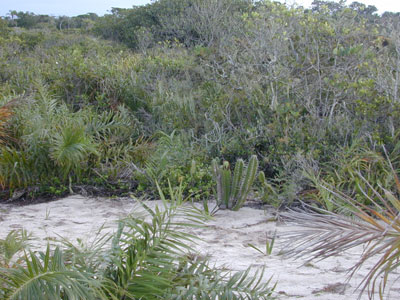
The coastal dune forest above represents a distinct plant community

Lecture 16 Communities - Structure and Dynamics

Email me

Back to:

Overview - Link to Course Objectives

• Community vs. Aggregation  (16 Intro, section 16.9, section 18.10)
• Diversity  (16.1)
  • Dominance Indices
  • Information Indices
• Diversity Factors  (17.6 and 17.7)
• Interactions among community members (17.2)
  • Indirect interactions   (17.3)
• Dominance  (16.2)
• Keystone Species  (16.3)
• Food Webs  (16.4)
  • Connectance
  • Food Web Generalizations
  • Trophic Structure
  • Top-Down and Bottom-Up Effects  (17.4)
  • Trophic Cascades and the Ecosystem Exploitation Hypothesis
• Guilds  (16.5)
• Physical Structure (combine 16.6 and 16.7 and 16.8)
  • Edge Effects  (17.5)

Community Definition (16 Intro and section 16.9)

• Community - a set of interacting species
  • This implies that they occupy some common habitat
  • Community has emergent properties dependent on the interaction of the populations living in it.
  • A community is usually a subset of the species occupying a particular habitat
    • can be all the species at a particular trophic level (all of the plants in a field, all of the carnivores in a pond)
    • can be all of the species belonging to a taxonomic group (I study all of the yeast in the cactophilic habitat)
• Assemblage - set of species occurring in the same place
  • a collection of populations of different species all living in one place because the environment has the correct resources (food, etc.) and physical properties (temperature, etc.)
  • no interaction is implied
  • Assemblages have few emergent properties due to the lack of interactions
• Question is always - am I dealing with a community or an assemblage?
  • The original community ecologists felt that the community was like an organism, in which the species were like the organs or tissues in an organism, and the community had its own set of properties, like the physiology of an organism.
• this is now felt to be an overstatement of the strength of interactions between species in a community, in general
• for an organism, the idea of emergent properties is not controversial, as we can do many more things as an organism than our individual organs can do
• The organism concept persists as the community concept - emergent properties from species interactions
• Community Emergent Properties are not just the sum of the abilities of individual species measured in isolation, but are the aggregate properties of more than one species and depend on the interaction between species
  • Trophic structure in an emergent property of large scale communities
  • One might study an assemblage by studying each species in isolation
  • One can only study a community with all relevant species present

Diversity - Richness and Evenness (16.1)

How are we to compare two communities?

• The simplest way might be to compare the number of species
  • Species Richness - The number of species in a community
    • Simply looking at species richness loses almost all of the information (types of species, numbers of each, relationships, etc.) we might use to compare the communities but is easiest to do.
  • Species Richness is usually estimated from a sample of individuals from a community
    • A problem arises because the number of species in a sample will depend on the size of the sample
      • Larger samples have more species
      • This is because not all species have the same probability of being in a sample because some of the species are common (high probability) and some are rare (low probability)
        • Small samples have common species and few rare species
        • Larger samples pick up more rare species
      • So, when comparing the Species Richness of two or more communities, you must correct the estimate of Species Richness from samples for differences in sample size (this is not necessary where sample sizes are equal)
      • The process of making the correction is called Rarefaction and a brief introduction to a method of rarefaction (there are many ways to skin this cat) can be found here
• To much detail might make every community look unique and obscure common features between communities
• Diversity (Biodiversity) uses more information that species richness
• Need a way to measure diversity
  • Example - compare two lakes in North America with one in Argentina
    • Both have similar abiotic characteristics
    • Can differ in the number of species present
    • Can differ in the evenness of the species present
  • Which of the below is the most diverse community??
    • Notice that the overlap in species differs quite a lot, as the Argentine lake shares no species with those in North America

• Not so easy to decide is it?

• Must include both a Species Richness component and a Species Evenness component
• There is no one way to measure diversity, so we will look at more than one

• Dominance Indices - examples: the Simpson and Berger-Parker indices
  • In dominance indices, the most common species make the greatest contribution, and adding lots of rare species will not increase the index's value by much
  • Berger and Parker proposed a simple index which is the total number of individuals of all species divided by the number of individuals in the most common species. Adding species (which must increase the numerator) will increase the index's value

    

    • Notice that this is the RECIPROCAL of the formula presented in the textbook so that the index will increase as the diversity of the community increases
      • If one were to use the formula as presented in the book (Nmax over N), the advantage there is that the index goes from 1 (least diverse) to 0 (most diverse) and this restricted range might be useful in an index
    • In this index, the addition of more rare species does not change the denominator but will increase the numerator (in the formulation above)
  • Simpson's index is simply the probability that any two individuals chosen randomly from the total population come from the same species. Each term of the summation is the probability that two individuals chosen randomly will come from a particular species and the summation gives the probability for all species.  This index can be used (as can all of these indices) with measures of density involving biomass or coverage area (from quadrat maps of vegetation - easy to get now with satellite images).
    • If there are S species and n_i is the number of individuals of the i^th species and N is the total number of individuals, then Simpson's index (which = 1 - D) is:

  

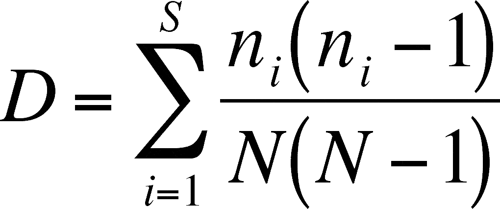
  • Notice that D will get smaller as the diversity of the community increases (if you keep N constant and increase the number of species, each ni must be smaller, on average, and so the numerators get smaller).
    • Simpson's index is normally expressed as 1/D so that the index will increase as diversity increases
    • Simpson's index uses information from each species, unlike Berger Parker, and so it is in some ways more accurate, but it is very insensitive (unchanging) to the addition of rare species to the sample

• Information Indices - the Shannon and Brillouin indices
  • This is a very different approach taken from the mathematical theory of information.
  • The rationale is that information is needed to characterize a community. How much?
    • Each individual needs to be included, but it there is less information needed if they can be grouped and tagged as a group.
    • So, if all individuals are different species, you would need a tag for each one (maximum information needed) and when all are members of the same species you need only one tag for all (minimum information needed).
  • Shannon index is a measure of the amount of information needed to describe every member of the community. If p_i is the proportion of individuals (from the sample total) of species i, then diversity (H') is:

  

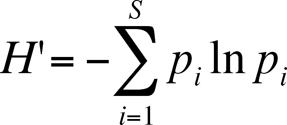
  • the negative out front is needed to offset the negative you get when you take the natural log of p_i (since p_i is a fraction, its log is negative)
  • as more species are included, the average p_i gets smaller and so its log get s more negative and the total value of the index increases
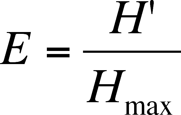
  • This is a useful measure because one can calculate evenness using it.
    • For any given sample size containing (N) containing S species, the value of H' will change when evenness changes. The maximum H' value (Hmax), without adding individuals or species, is attained when the numbers of individuals of every species is equal (here, the proportion would be 1/S). Evenness (E) is then the ratio of the actual H' value to the maximum value (and thus it ranges from 0 to 1)

  

  • In this index, both species richness and evenness matter.
    • When the number of species increases, H' increases.
    • When one species dominates (and evenness decreases), H' decreases.
  • The Shannon index is dependent on the assumption that the sample used to generate it is a random sample of the community

  • Brillouin Index
    • Useful when the randomness of the sample is suspect
    • Similar to H', but based on numbers instead of proportions

    

    • all of the symbols are as before
    • this index will increase as the total number of individuals in the sample increases, even if the number of species nor the species' proportions do not change
    • For more on the calculation of these indices, refer to the document "Diversity Index Calculation" by clicking on the blue link

Diversity Factors (17.6 and 17.7)

Environmental Heterogeneity

• as the environment becomes more diverse, so does the biological community
• as the diversity of one biological community increases, this might act to increase the diversity of other communities (more diverse forests have more diverse bird or insect communities)

Environmental Quality

• Environments rich in resources (nutrients for plants, long growing period, etc.) are more productive (greater total photosynthetic production) and usually support more diverse consumer communities
• Some exceptions are known
  • Plant communities on low nutrient soils are more diverse than those on high nutrient soils
  • With lots of nutrients, some species dominate the system and exclude others
  • may be due to Size Symmetry
    • root competition (for nutrients in poor soil) is size symmetric and large plants have only a proportional advantage in getting nutrients
    • light competition (get the light and shade your neighbors) is size asymmetric and allows taller plants to have a disproportional effect by not just getting more light but excluding their neighbors by shading them

Interactions among species within a community

• Direct Interactions are interaction in which a species affects another without the intervention of other species
  • predation, interference competition, herbivory, parasitism, and mutualism are all direct interactions
• Diffuse Interactions (17.2) are interactions with other species that have small effects on a species-by-species basis
  • Diffuse interactions can have an important cumulative effect
  • Diffuse interaction can be either direct or indirect
• Indirect interactions (17.3)
  • effect of one species on another mediated through the presence of a third species
  • examples of some indirect interactions (also known as indirect effects)
  • Competition x Competition
    • consider three species, A, B, and C. C out competes B, but not in the presence of A. B out competes A. When all three species are present, C cannot out compete B due to the presence of A
  • Competition X Mutualism
    • Two competing species may have the outcome of competition altered when mycorrhizal fungi are present
  • Predation X Parasitism
    • parasites can increase predation by stressing the prey and making them more vulnerable to the predator
    • thus, parasitism of the prey can increase predator population size (indirect effect of parasite on predator)
  • Predation X Competition
    • predators can feed on the most common prey
    • this can reduce the ability of a competitive dominant species to oust its competitors
    • this sort of indirect interaction where the loss of the predator causes weak competitors to disappear from the system is called Keystone Predation
  • Competition X Parasitism
    • A competitive dominant species can be weakened by the presence of a parasite so that it cannot oust species that are its competitive inferiors (remember the flour beetles and the effect of the protist parasite)
    • This can also result in Apparent Competition
      • Species A carries (and tolerates) a parasite that can kill species B
      • When species A is present, species B disappears, which looks like competition
      • Cases where competition seems to be the mechanism but another process mimics the outcome of competition are called apparent competition

Dominance (16.2)

• Species are not distributed evenly and a few species may contribute most of the individuals (or the biomass, where individual size varies greatly among species).
• Dominance is not strictly the converse of diversity, for a community can be diverse and have dominant species if there are many rare species present.

• Dominance is the converse of evenness, the second contributor to diversity.

Keystone Species (16.3)

• Keystone species are those with a disproportionate effect on the community. 
• The impact may come through:
  • competition - some species may be able to exclude others, so that when the best competitor is removed, several species can invade
  • predation or herbivory - removal of a predator or herbivore that feeds on the best competitor in a community may allow the that competitor to expand its population size so that it competitively excludes other species.
  • keystone species may be prey as well as predators
    • loss of a keystone prey species results in loss of many predatory species
  • structure - some species may alter the environment in a way that creates opportunity of other species
    • trees become habitat for many animals
    • corals build reefs that become habitat for many algae and animals
    • Beavers are a classic keystone species that act as ecosystem engineers
      • Alter the environment by building their homes by making ponds
      • hundreds of species in the ponds rely on the presence of the beavers
• They may be dominant species but it is not necessary that they be dominant

Food Webs (16.4)

• Food Webs are based on which species eat other species.
  • This may be directly (predation, herbivory, parasitism) or after the food item is dead (detritivory)
• Simple interactions are Food Chains but more realistic maps of interactions are Food Webs
• Remember that this view of a community is based on feeding and that there are other relationships between organisms that are not part of a food web
  • habitat formation, competition, amensalism, commensalism are examples of non-food web interactions
  • pollination when no food is consumed is another
• Connectance: - The Math of Food Webs
  • Trophic link - relationship between a pair of species indicating that one eats the other
  • Connectance - the ratio of actual links to the total number of links possible for an ecosystem
    • Interest in this comes from the idea of stability
      • Some believe that interconnected systems are more stable
      • Others believe that as interconnectivity increases, instability increases
    • Connectance = number of links/total number of links possible
      • If n = the number of species in the web, the total number of links possible = (n[n-1])/2
      • Low ratio means that species eat relatively few other species and the food web is simpler
      • High ratio means that species eat lots of other species and the food web is complex
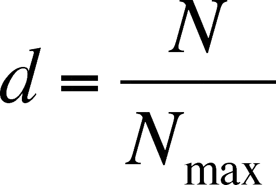
    • Linkage density (d) - average number of links per species
      • d = total number of links/number of species
      • a second way to look at food web complexity (only partially correlated with connectance)
      • as you add species, if d remains the same, then connectance will fall
    • There is no agreement about how connectance and linkage density change with an increase in the number of species
• Generalizations about food webs
• Omnivory is rare and links usually do not form circles
• Because this is so, we can define Food Chain Length as the average number of links between producer and tertiary consumer in a food web
• Food chains lengths tend to be short
• Food chain length does not correlate well with total productivity of the system
• Food chain lengths are shortened by:
  • Island size (smaller islands have shorter food chains)
  • Human disturbance (disturbed habitats have shorter chains)
  • Habitat complexity (longer in complex habitats)
  • Chains are shorter in two-dimensional habitats (grasslands, organisms attached to hard substrates) than three dimensions (forests)
• Objections to the generalizations
• We almost always have incomplete information on food webs
  • Often we aggregate (lump) species that look similar without knowing if their diets are really similar
• The theory does not make any adjustment for the importance of a species in another species diet
  • If most of the species in a diet are just occasional snacks, the food web is actually simpler than the map of trophic links indicates
• Limiting nutrients are not usually known
  • Minor links can be critical if they supply limiting nutrients

• Trophic Structure - (trophic refers to feeding) - generalized depiction of a food web with many species lumped together into a level (therefore, the structure becomes a hierarchy)
• Basal level - Primary Producer - autotrophs (Photoautotrophs and Chemoautotrophs) - fix inorganic carbon into organic compounds and utilize a source of energy other than that found in organic molecules
• second level - Primary Consumer - organisms that feed on the primary producers, such as herbivores
• third and more levels - Secondary consumer - predators that feed on primary consumers (third level) or on other predators (4th and subsequent levels)
• Problems with the trophic hierarchy:
• many organisms feed at more than one level
• parasites, Transformers, and decomposers (detritivores) not really a part of the system in a hierarchical way
  • More primary production may be consumed by detritivores than my herbivores in many systems.
  • Decomposer is another word for detritivore - they catabolize complex organic detritus - fungi, insects and bacteria feeding on leaf litter, scavengers of dead animals
  • Transformers live by altering nutrients from organic or reduced to inorganic or oxidized forms (or vice versa) - denitrifying bacteria, nitrifying bacteria
• Trophic Pyramid - Inefficiency in energy flows between levels of the trophic hierarchy mean that the size of trophic levels (in numbers or biomass) decreases as you go from primary producer up the hierarchy, which usually gives trophic level histograms the shape of a pyramid
• Energy pyramid is always broadest at base
  • Outcome of second law of thermodynamics
• Biomass pyramids usually wider at base, but can be inverted
  • When turnover is high, biomass can be small, but productivity is still high
• Top-Down and Bottom-Up Effects (17.4)
• The hierarchical nature of trophic structure may have an effect on the kind of interactions that regulate populations
• There is no agreement on how tropic interactions will affect population regulation and two general types of interactions have been proposed:
  • Top-down effects means that the top of the food web sets the size of populations lower down the chain
    • Predators (high on trophic pyramid) regulate prey populations size (prey are, by definition, on a lower level than their predators)
    • Example of top-down effect
      1. Increase in number of predators subsequently -
      2. Reduces size of herbivore population which -
      3. Increases size of plant population and this -
      4. Reduces nutrients in soil
  • Bottom-up effects means that the bottom of the food chain sets the size of populations higher up the chain
    • since each tropic level derives its energy from the level below it (and some of that energy is lost to heat in the transfer process - think second law of thermodynamics), then the productivity of the species on the lower layer sets the bounds on the population sizes of the species on the higher layer
    • Example of bottom-up effects
      1. Increase nutrients in soil
      2. More nutrients increases size of plant population
      3. More plants increases herbivore population
      4. More herbivores increases size of predator population
• Field examples of both are known, so we are not able to decide which is more important at this time

Trophic Cascades When the size of a population is affected by the size of populations on trophic levels more than one step removed from it, then these interactions are called a trophic cascade

• can result from both bottom-up and top-down effects (see examples above)
• one general hypothesis about communities based on trophic cascades is the
  • Ecosystem Exploitation Hypothesis combines elements of both top-down and bottom-up regulation
    • most important variable is the total productivity of the primary producers
      • when primary productivity is low, there is not enough production of biomass to sustain large herbivore populations
      • as primary productivity increases, herbivore populations increase
        • thus most of the increased production winds up as herbivore biomass, not primary producer biomass
      • as primary productivity increases still more eventually the herbivore populations are large enough to support prey populations
        • predators depress herbivore population sized
        • fewer herbivores increases biomass of primary producers

Guilds (16.5) are groups of species that all utilize a resource in the same way so that their interactions are characterized by the effect of the shared resource

• simplifies the approach to studying the community
• often a trophic interaction that characterized a guild
• all seed-eating birds in a forest
• all insects that feed on oak by mining its leaves
• all parasites that parasitize parasitoids in an area (these are called hyperparasites since they parasitize parasites)

Physical Structure of Communities (combine 16.6 and 16.7 and 16.8)

• Communities are both the species interactions and the physical structure that those species produce
• Forests are more than collections of trees - they have different Zones within
  • Canopy (upper layer of leaves that get direct sunlight)
  • Understory (shaded plants underneath the canopy)
  • Herb Zone (grasses and non-woody plants near the forest floor)
  • Forest Floor (layer of loose detritus atop soil)
• Whenever physical structure changes in a regular way you get Zonation
  • examples
    • the regular changes between a pond and the adjacent forest
    • the regular changes between tidal creeks and the adjacent shrub community in a salt marsh
      • (Tidal Creek, Tall Spartina, Short Spartina, Juncus, and Shrub Zones)
    • the regular changes between valley forests and bare rock at the top of tall mountains
  • Transitions from one zone to another are often gradients and so the edges are hard to define
    • usually marked by changes in both physical factor (moisture, temperature, light) and by a change in species composition
  • Edge effects (17.5)
    • species composition can be altered by
    • Stress - species disappear because the new zone is too stressful
    • Competition - species are excluded from adjacent zone by other species

Terms

Community, Assemblage, Species Richness, Dominance Index, Berger and Parker index, Simpson's index, Information Index, Shannon index, Evenness, Brillouin Index, Environmental Heterogeneity, Size Symmetry, Direct Interaction, Diffuse Interaction, Indirect interactions, Keystone Predation, Apparent Competition, Dominance, Keystone Species, Ecosystem Engineer, Food Webs, Trophic Link, Connectance, Linkage Density, Trophic Structure, Primary Producer, Primary Consumer, Secondary consumer, Trophic Pyramid, Decomposer, Transformers, Top-down effect, Bottom-up effect, Trophic Cascade, Ecosystem Exploitation Hypothesis, Guild, Canopy, Understory, Herb Zone, Forest Floor, Zonation, Edge effect

Last updated March 9, 2007