BIO 412 Principles of Ecology Phil Ganter 301 Harned Hall 963-5782
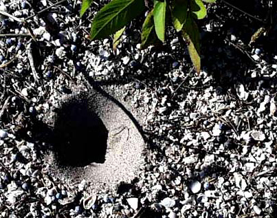
Antlion pit - an antlion (not visible) is a lacewing larva

Spatial Patterns

Email me

Back to:

Introduction: In this lab, we will go to a forest and not measure many of the things one might measure there. We will not, for instance, measure the density of trees or their average size, or the diversity of species. Hopefully, we will get some idea of this from simply walking through the forest and being observant. These are all important things to know, but they may not tell one much about the interaction among trees, which is what I would like us to concentrate on today. We will look for patterns in space. For sessile organisms, like plants or corals, the environment in which they develop and reproduce can not be changed once they germinate (or settle out of the water column). Their environment is the immediate neighborhood. The neighboring trees are potential competitors, whether or not they are of the same species. When we observe such organisms, it may be possible to detect some interactions from their spatial pattern. Before we can do this, we should consider what patterns might be there and what they might mean.

If trees do not interact, the location of any tree would be independent of the location of any other (assuming that they fall to the ground independently too). This would lead to a random spacing of trees. A second possible pattern might be that trees are spaced evenly (like corn plants in a field). This pattern can be called either uniform, regular or "under-dispersed." Ask me during the lab how that last name came about. One thing that could give rise to regular spacing might be some kind of competition, such that there is a minimum distance between plants, as each plant commands the resources (light, moisture, nutrients) within its sphere of influence and this keeps other plants from growing there. A third possible pattern might arise when plants find the underlying substrate uneven in quality. If this is so, many plants may cluster within the patches of good quality, giving rise to short interplant distances within the patch, while distances between plants in different patches would be large, separated by the poor patches in between them. This would lead to two kinds of distances, very large and very small (with few intermediate distances). This pattern is called aggregated, contagious, clumped or "over-dispersed". There are many possible reasons for aggregated distributions other than patchy resources. Remember that I assumed a random seed fall when describing how random dispersion patterns arise. However, if a plant depends on an animal to disperse its seeds, then the behavior of the animal when doing so might lead to aggregated distributions. Other factors such as storms, disease, and insect infestation might also lead to clumping. Here is a challenge. Can you suggest another reason for a regular dispersion pattern other than interplant competition (other than human intervention)?

While pattern analysis is not a definitive proof of interaction (one would have to do an experiment to determine the real cause of the patterns), it is useful as a means of generating testable hypotheses about the interactions between trees. We will take an experimental look at the interaction among plants in another lab. In addition, we must remember that spatial pattern is important to all populations, without regard to the organisms that comprise the population. The antlion pit pictured above is made by a tiny monster that digs a pit and lies in wait at the bottom to poison and eat whatever smaller insect falls into the pit and can't climb out. The pattern of other antlion pits in the neighborhood has a strong impact on the number of prey the antlion will get, and so antlions have been shown to alter the spatial pattern of their pits as the local density of antlions changes.

Gathering the Data:

Sampling Design:

When confronted with an object of study as large as a forest, or even a single species within the forest, it is rare that one can census the entire population. Therefore, what one must do is sample a subset of the entire population and draw conclusions about the whole from the sample. There are many ways to do this, and we will look at two today, quadrat sampling and transect sampling. Quadrat sampling subdivides the area into smaller blocks (= quadrats) and samples some of them. Transect sampling (of which there are many versions such as linear intercept, point-quarter, and the one we will use today, nearest-neighbor) samples only those individuals that occur at pre-determined points along a line(s) (= transect(s)) through the sampling area.

A second consideration is whether or not one should stratify the sampling area. Unstratified sampling treats the entire area as unchanging or all individuals as equals. This might be true in cases where the there is little change in elevation or soil type within the area or in cases where individuals of all species and ages have similar resource requirements. Many times, one can easily see that there is a change in elevation or one may have a map of soil types within the area. There may be a physical feature which can obviously affect one side of the area of interest more than another (such as a river along one side). Mature individuals may use different resources than immatures or species may have different resource requirements. When this occurs, one can choose to stratify the sample, which means to subdivide the sampling so that some samples are taken from each of the different strata (low and high elevations, chalky and loamy soils, wet and dry soils, large and small individuals, different species). We will stratify our sampling into just two categories of trees: canopy trees and understory trees. Canopy trees are those trees that are not shaded by other, taller trees. Sometimes a canopy can be closed, by which I mean that there are no gaps large enough so that shorter trees can join the canopy merely by growing taller. Not all forests have a closed canopy (those without a closed canopy would have an open canopy). Understory trees are smaller trees that do not have direct access to sunlight because they are shaded by older, taller trees.

Quadrat Sampling of a Forest:

One must make four decisions in order to do quadrat sampling.

How large should they be?

• This is a practical decision. The quadrat must be large enough so that more than one individual can reasonably fit into it and not so large that one can not count enough quadrats to adequately sample the population or forest. We will make our quadrats 12 m by 20 m.

How many quadrats are to be sampled?

• Once again, this is a practical decision. There are eight groups in the class, and each will sample two quadrats for a total of 16 for the class.

How are we to count the individuals within a quadrat?

• This decision is not simply a practical one. One may wish to consider all of the trees sampled as equivalent, so that one simple counts the number of stems of each species of interest. Often, the size of the individual is important.
• For trees, size can be considered from two perspectives. The amount of sunlight available for a forest plant is related to its height. Plants in the forest canopy receive direct sunlight, those below are shaded by the canopy plants. The amount of nutrients and water available to a plant is related to its cover area, the area of its crown of leaves (which is usually assumed to be circular).
  • For small, understory trees and shrubs, this is measurable directly.
  • For canopy trees, the basal area of the trunk (cross-sectional area at a pre-determined height from the ground) is substituted as it is usually directly related to the crown size above.
• However, for our purposes, we will stratify our sampling into canopy and understory trees and simply count the number of stems in each category. You will have to decide if the tree is in the canopy or not.
  • A practical consideration: If any part of a plants stem is in the quadrat, it is counted.
  • Another practical consideration: We will ignore all plants that are less than 1 inch in diameter at breast height (often abbreviated dbh).

How are the quadrats to be placed within the sampling area?

• There are many ways to do this, and we haven't the space to describe them all or even a reasonable subset. However, two things should be mentioned.
  • Often one maps the entire area, divides it into square coordinates (like latitude and longitude on large maps) and randomly picks the coordinates at which the quadrats are placed.
  • A second commonly used method is to use a transect to locate the coordinates by randomly choosing points along the transect to place the quadrats. We will use this method, since our study area (called Tornado Ridge) has a natural transect, the trail along the top of the ridge. We will locate our quadrats along the ridge at (pseudo)randomly chosen points.

Your data should take the form of a table, with category of trees found along one side as the rows and quadrat number along the top as columns.

Nearest-Neighbor Sampling:

• This technique is based on one or more transects of the sampling area. We will do a single transect and all will use the same transect. You will sample at one point and then leapfrog the rest of the class to go to the next point on the transect to collect some more data. Collect data from at least 3 transect points.
• The procedure is to walk along the transect and stop at random points. Choosing a minimum spacing that will guarantee that no tree is sampled at two consecutive transect points.
• At each sampling point, divide the world into four quadrats by drawing a line on the ground (with your shoe is fine) along the transect and then crossing it with a second line at right angles to the first. they should cross at the transect point. For both canopy and understory pairs, you will measure a nearest-neighbor pair in each of the four quadrats (8 pairs at each transect point)
• In each quadrat, determine the nearest canopy tree. You may have to measure the distance between a couple of trees and the point to determine which is the closest.
• In the northwest quadrat, find the nearest neighbor to that tree (measure more than one tree if you can't tell which neighbor is nearest by eye). The nearest neighbor must be another canopy tree.
• Record the distance between nearest-neighbors.
• Measure the basal area of both neighbors. We will measure the basal area of canopy trees by wrapping a measuring tape around it at breast height to get the circumference. Later, you can convert this to basal area with the formula below
• 
• In the same quadrat, repeat the procedure for an understory tree, so that you have collected data from one nearest-neighbor pair of each type of tree (1 understory pair and 1 canopy pair) in that quadrat. Be sure to take down the circumference of each tree and the distance between each.
• In the Northeast quadrat, find both nearest-neighbor pairs. A work of caution. You always start with the tree nearest to the transect point and work with its nearest neighbor. This might mean that the nearest neighbor is a tree already sampled when working on an earlier quadrat. This is OK. Just don't violate the rule about starting with the tree closest to the transect point. The nearest neighbor might also be a tree in another quadrat (will often be so). This is also OK, just don't violate the rule about using the closest neighbor, no matter where it is located.
• Do this for at least 3 transect points (i. e., for 3 stops). Once again, ignore any understory trees less than 1 inch dbh. This will give you a total of 24 nearest neighbor pairs (12 canopy, 12 understory).

Data Analysis:

One of the ways in which organisms may interact is competition. Competition has long been of interest to ecologists because it may explain many patterns (spatial and other types) observed in natural populations and communities. Let's see if we can't detect it in our sample by making some assumptions about what spatial patterns might be the result of different interactions between organisms.

Quadrat data:

The three patterns (regular, random, and aggregated) can be easily detected with a statistic called the variance-to-mean ratio. We can symbolize this as ²/. The symbols are the standard statistical notation (Greek is used for a particular purpose by statisticians): is sigma and sigma squared is the variance, is mu and is the mean. First, you should organize you data into a frequency distribution of individuals per quadrat. Some quadrats will have contained 0 or 1 or 2 or 3 or more trees. For example, suppose that 4 quadrats had 2 trees, 6 quadrats had 3 trees, 5 had 4 trees, 2 had 5 trees, 4 had 6 trees and one had 8 trees. Then the we can then group the data as:

Note that x_i refers to the number of trees in a quadrat and frequency is the number of quadrats that contain x_i individuals. You can construct a frequency diagram by hand or can enter the raw data and use the skills you learned in the lab on spreadsheet graphics to have the computer make the frequency table from the raw data. This will eliminate counting errors.

You can easily calculate the mean from such a table. I will do it for the above table, you have to use your table.

• First, add up all of the frequencies. This is the total number of quadrats.
  • Number of quadrats = sum of frequencies = 4+ 6 + 5 + 2 + 4 + 1 = 22
• Then multiply each x_i times its frequency and sum all products. This is the total number of trees in all quadrats.
  • Number of trees = sum of (frequency x x_i ) = (4·2)+(6·3)+(5·4)+(2·5)+(4·6)+(1·8) = 88
• Now divide the total number of trees by the total number of quadrats and you have the mean trees per quadrat. This is half of the statistic.
  • Mean = = 88 / 22 = 4.0

xi	Frequency	xi x Frequency	xi -	(xi - )2	(xi - )2 x Frequency
2	4	8	-2	4	16
3	6	18	-1	1	6
4	5	20	0	0	0
5	2	10	1	1	2
6	4	24	2	4	16
8	1	8	4	16	16
Totals	22	88			56

You also need the variance. This is a measure of the spread of the actual data around the mean you just calculated. To calculate this, you need the data and the mean, so variance can only be calculated after the mean.

To calculate variance:

• subtract the mean from each of the x_i values
• square each difference
• multiply the squared value times the frequency
• sum these products
• divide the sum by the total number of quadrats minus one.
• Variance = 56 / 21 = 2.67

The variance-to-mean ratio is: ²/ = 2.67/4 = 0.67

Now, why do we calculate such a statistic? It can be shown (we haven't the space here) that the three types of patterns all have different variance-to-mean ratios. So, the statistic can be used to infer the underlying spatial pattern. If the pattern is random, then the variance is equal to the mean and v/m is 1. If it is aggregated then s/m is more than 1. Remember that we get more small (when the quadrat has no clump of trees) and more large (when the quadrat is in a clump of trees) tree counts than expected when the trees are clumped. It is the large values that make the variance larger than the mean because you square the differences when calculating the variance and large differences result in big square terms. Finally, uniform or regular patterns have a variance-to-mean ratio less than 1. Things that are equally spaced out have little differences among tree-to-tree distances and so every quadrat contains the same number of trees and there the variance is very small.

So, we can see that our statistic is telling us that this population is underdispersed or regularly spaced in our example. The trees might be competing. However, there is one little problem. If the population were actually randomly spaced and we took a sample, we could not expect that the sample data would give us a ratio of exactly 1. It would be like flipping a coin a hundred times and betting your life that you get exactly fifty heads. Although we expect to get 50 heads, it is still a bad bet. Random chance can cause deviations from expectation. In our example here, the question is, "Is 0.67 an indication of regularity or is the real value 1 and we measured 0.67 due to some experimental error?". Put another way (as a statistician might ask it), "Is 0.67 significantly lower than 1? Well, there is a way to infer whether it is or isn't!

Using the Poisson distribution to predict what data a randomly spaced population of trees should have given us

So, what would we expect if the distribution in our sample came from a randomly spaced population? We don't want to change the mean number of trees per quadrat. We just want to know if our data is within reason, given the mean, or is our data so different from the data we would have expected to gather from a randomly spaced population that we can't accept that the difference between observed and expected is due to random error. There is a mathematical way to calculate the expected distribution of trees per quadrat given our mean and a total of 22 quadrats (the number of quadrats may differ in your data). This distribution is called the Poisson Distribution and is worth learning as it predicts random outcomes from any data that can be summarized with a frequency table. According to the Poisson, the proportion (= percentage) of the quadrats one should expect in any class (= x_i) can be calculated from the following simple formula.

Proportion in xi =

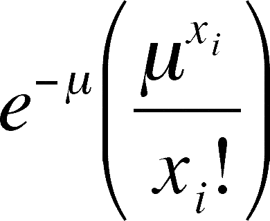This equation may be rather daunting, but I will walk you through it. The only new symbol is e, which is the base for natural or Naperian logarithms and is about 2.718 or so. Suppose you are trying to calculate how many quadrats you expect to get with 5 trees in them in our example (22 quadrats, mean of 4 trees per quadrat). First, you raise 4 (= m, the mean) to the 5th power (5 = x_i) and divide this by 5 factorial (= 5 times 4 times 3 times 2 times 1 = 120). Then you take this quotient times e (= approx. 2.718) raised to the negative 4^th power. Simple, right?

Proportion of quadrats with 5 trees =

The answer, 0.156, means that about 16% of the quadrats should have 5 trees. This is about 3.45 quadrats (= 22 quadrats x 0.156, remember that fractions are ok when you calculate them, although 0.45 of a quadrat doesn't really exist). In the table below are the complete set of expectations for our data. The expected number of quadrats is gotten by multiplying the expected proportion of quadrats times the total number of quadrats. The observed number comes, of course, from the raw data (look at the table above)

• Notice that the sum of all the expectations equals 22. We can't expect any more or less than the total number of quadrats we actually sample. The problem is that the Poisson distribution goes to infinity, although we never got a quadrat with more than 8 trees. So, I lumped all of the classes above 8 in with 8 (notice the 8+) and this makes the proportion of quadrats expected in this class easy to calculate. Simply add the preceding classes together and subtract the sum from 1.
• Notice that for some of the classes (the x_i's) that we expected to get something, even though we didn't actual see any quadrats with that number of trees (as in 0, 1 or 7 trees/quadrat). You can't ignore a class simply because you didn't happen to get any data there!
• Finally, recall that 1! and 0! are equal to 1.

xi	e-	xi	xi!	expected proportion	expected number	observed
0	0.018	1	1	0.018	0.4	0
1	0.018	4	1	0.073	1.6	0
2	0.018	16	2	0.147	3.2	4
3	0.018	64	6	0.195	4.3	6
4	0.018	256	24	0.195	4.3	5
5	0.018	1024	120	0.156	3.4	2
6	0.018	4096	720	0.104	2.3	4
7	0.018	16384	5040	0.060	1.3	0
8+				0.030	1.1	1
			Totals	1.000	22	22

Important Pause:

Ask yourself this. Am I sure that I know why both the expected number and observed columns sum to 22 and why the expected proportions sum to 1? If you do not, you are confused about this table and should ask your instructor for clarification. Notice that I had to calculate the expected proportions and numbers for 0, 1, and 7 trees per quadrat, even though I did not observe any quadrats with those trees. This can be a nuisance when you get one or two very large observations with a lot of zero entries in between (consider a situation where one quadrat had 25 trees. I then have to calculate all of the categories between 8 and 25, although there is no data in these categories). This is when it is best to do the calculations with a computer spreadsheet program or to lump the categories from 8 to 25 into one category. Notice that the last category is 8+, not just 8. The expected number of quadrats with 25 trees is part of the lumped category (as is the number of quadrats with 250 trees, 2500 trees!). The Poisson distribution is infinite, and assigns probabilities to all values of xi greater than 8. The last category in a Poisson table always lumps the categories to infinity.

As you can see, there is some discrepancy between the observed numbers of trees per quadrat and the expected numbers if the trees were spaced randomly (remember that the Poisson assumes the trees are randomly distributed). But, to get back to the central question, is this a significant difference between random expectation and our data? If not, then the distribution of the trees in our example is random. If the difference is significant, then the results are different from results expected from randomly spaced trees and the trees in our example are regularly spaced (because the s²/m ratio is less than 1). So, how do we decide on significance? This is subjective, so I as lab instructor will make a decision. A difference is significant if there is less than a 5% chance that the actual (observed) data would be so different from the expected results if the trees were distributed randomly. So, now to the determination of just how likely the example's statistic (v/m = 0.67) is if we assume the actual pattern is random.

Using the Chi-square test to decide if observed and expected results differ significantly

We will use a statistical technique called the Chi-square test (²) to figure our chances. Its calculation is easy.

• For each x_i, we have an observed and an expected value.
  • subtract the expected from the observed
  • square the difference
  • divide the difference by the expected value.

The squared difference (column 5 below) is a measure of how unexpected the data are (given the assumption of randomness) and dividing this by the expected value corrects for the fact that some data comes in ones, some in tens, some in hundreds, etc. Without this correction, we could not use the same test on data that comes in large values (like bacterial numbers) and data with small values (like tree quadrat data). The Chi-square value is the sum (for all x_i) of these quotients.

In order to evaluate this result, you have to use the table at the end of this lab (or from any standard textbook) or you can use MSExcel. You can read the probability of your results differing from expected results due to only random error from this table (ask your instructor how to use the spreadsheet program).

• First calculate the degrees of freedom, which is the number of categories (the number of x_i's) minus 1 (9 - 1 = 8 in our example, remember that the 0 class adds one, so we start with 9, not 8).
• Your results are significantly different from random if your Chi-square value exceeds the one in the table at the end (this table includes values for the previously chosen 5% decision making rule as well as two more strict values. Use the 5 % column).

Since the value in the table is 15.5 and the value in the example is 6.2, we can conclude that we do not, in fact, have evidence that the spatial distribution of trees in our example is regular. Although 0.67 seems very much smaller than 1, gathering 22 quadrats with a mean of 4 trees per quadrat from a forest in which the trees were spaced randomly would give such a low value (through random error when taking the sample) more than 5% of the time.

What your assignment must have

• Present the class frequency table
• calculate and present the mean, variance, and variance-mean ratio
• calculate and present the Poisson expectations for the data
• calculate and present the Chi-square value and tell what your conclusions are:
  • what does the Chi-square value mean?
  • how are the trees distributed?
• Draw conclusions about competition between canopy and understory trees based on the data and the statistical probabilities calculated.

As a matter of fair disclosure, I must tell you that the conclusion you have reached is based on the size of the quadrats. A different quadrat size might lead to a different conclusion. However, we will only discuss this among ourselves and will not worry about it when drawing conclusions about our data.

A last note about the statistics calculated here. Many statistical tests work better with large amounts of data than with small amounts. Both the Poisson and Chi-square calculations are subject to some error when the data in any category is too small. The rule of thumb for both is if any calculated expectation (expected number of quadrats) is less than 5, one normally combines x_i's so that all expected values exceed 5. We might have done this here by grouping the x_i's. However, we may have so little data here that this would not be particularly useful, so we will simply ignore this for this lab exercise.

Nearest-Neighbor data:

Let's just rehash how we are looking for some evidence of competition among trees with the nearest-neighbor data.

• If we think of plant competition being based on gathering all of the resource within an "area of influence" then larger plants will have a larger area of influence than do smaller plants.
• A second assumption we need to make is that the areas of influence of competing plants can not overlap because one plant will remove the resource and leave the other plant at a disadvantage. Non-competing plants might have overlapping areas of influence, as neither can exclude the other.
• A final assumption is that the size of the basal area of a plant is related to that plant's area of influence.

With these assumptions, we can look for competition. If you understand the logic, you should be able to answer the question:  If the trees are competing, what should happen to nearest-neighbor distances as the neighbor trees get larger?  The distance should get ....  I leave it for you to fill in.  But we must base any conclusion we come to on our data, which requires that we analyze it for evidence of competition.

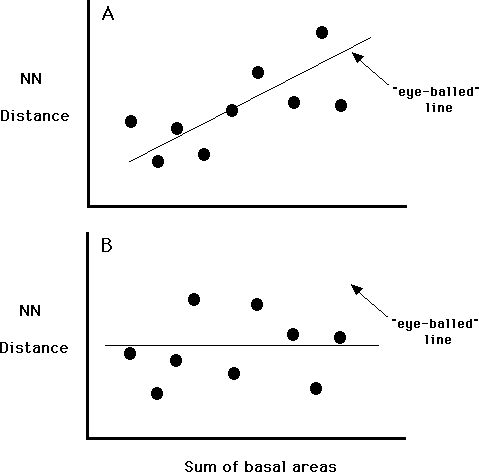
Drawing a line to represent the relationship between the nearest-neighbor distance and the combined size of the nearest neighbors
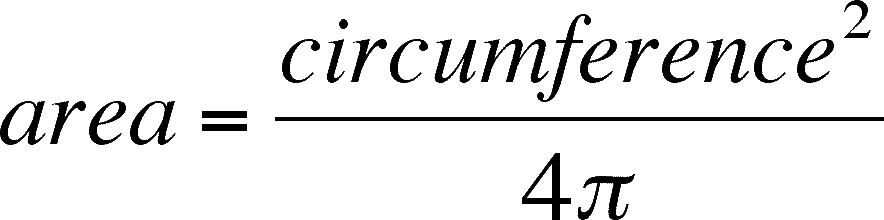
You should have the following data:  a set of nearest-neighbor distances and, for each NN distance, a total area (= sum of the two areas of the nearest-neighbor pair of trees).  Look at the data.  Use Excel to make a graph of these two variables.  Does it appear that there is a trend in the data? This can be asked a second way. As the combined size of the pair of trees increases as we go out the x-axis from the origin, does the nearest-neighbor distance tend get larger, get smaller, or not change? Notice I said "tend to get" because we expect random factors to affect the data and so the graph will be messy.  How can we describe and measure the tendency?  Since algebra I in high school, you have been taught that a line (curved or straight) represents a function or relationship between x and y.  We need to find a line that will describe the relationship between the nearest-neighbor distance and the combined size of the nearest-neighbor pairs.  We can use this relationship as the basis of drawing a conclusion about the presence or absence of competition between canopy trees (or understory trees).  Take a moment and think about what I just said. If you can see why the previous statement is true, proceed. If not, you need help and need to talk with your lab or lecture instructor.

So, how can we come up with a line?  First question: should it be a straight line or a curved line? Well, the equation for straight lines is simple and you have worked with it more than with any of the equations for curved lines.  The simplicity of a straight line means that Occam’s Razor (don’t know it? Google it.) encourages us to prefer the straight line unless we have some reason for expecting a curved (also called a non-linear) relationship. That said, we will use a straight line for our data.  But which line is best?  There are several ways of getting our “best” straight line.  One is to make an eyeballed estimate with a ruler and drawing a line.  But is that the best line? (The lines in the Figure below are eyeball fits - are they the same as you would make?) Without some math, there is no way to know. What we must do is to “fit” a line. By fit, I mean to draw a line, measure how good it is, and compare it with other lines to choose the line that fits the best.

There are many different ways of doing this, some of which are very complicated and/or require a lot of computing power.  The method we will use is the most common for simple models like a linear model and is mathematically very simple.  This method is called least squares, and if you have taken a statistics class you will probably be aware of this method, at least in name if not in practice.  It is used in linear regression for fitting the equation of a straight line to data, but can also be used for more complicated curved models like the logistic or type II functional response.
Most statistics software packages have sophisticated algorithms for fitting models using the least squares approach, but we will build our own fitting routine in Microsoft Exel.  Open MS Excel (or go to a new worksheet in the one you created to do the lab or just go to an unused area on your open worksheet - I will assume you are using a blank worksheet in the instructions below).   Label the following columns in the top row (the capital letters refer to the letters at the top of the columns in the Excel file): A – Total NN Size, B - NN Distance, C – Predicted Distance, D – Squared Deviations, E - Sum of Squared Deviations.  Go down four rows in column E (cell E4) and enter the following word: Intercept.  Go down cell E7, three rows below the cell with “Intercept” in column E and enter the following word: Slope.

First, enter the data from the lab in columns A and B below the labels you entered. Column C is filled in by using the equation for a line: y = mx + b.  The x’s will be the total size (= summed areas) of the NN pairs from your data (that is, column A).  We will then predict the nearest-neighbor distance using the linear equation.  This will be done in column C.  To make the prediction, we have to enter a formula to take the data from column A, multiplying it by a slope (m) and adding an intercept (b).  You have to use the same values for intercept and slope for each row with an entry in column A.  These values will be held in the cells in row E immediately below the appropriate label.  I will describe how to do enter the equation for the first row with a number (row 2 because row 1 has the label in it).  I click on row 2 of column C (cell C2) and enter an = sign (needed to tell the program the cell will contain a formula) and, after the =, (E$8 * A2) + E$5 and then hit return.  You will get an error message but this is OK.  Remember, the $ in the formula means an absolute references so that, when you copy the formula into the cells below, they go to the same place for the slope and intercept.   You might have to change the cell designations to match your spreadsheet but, in my spreadsheet, E8 is where I will have my slope stored and E5 is where the intercept will be. Copy the formula into the rest of the cells in column C (you will get an error message in all of them).

Now enter values into the cells that hold the slope and intercept.  I always start with 1, but any value will do.  Notice that you get values replacing the error messages in column C.  These are the predicted nearest-neighbor distances based on column A and the linear formulas entered in column C.  How good is the match between the real data (column B) and the predicted data in column C?  You will make the match visible by making a chart below the data with the values in columns A, B and C as the source data.  Do this now , choosing the scatter plot option, and label the axes.  If you have selected the labels along with the data to make the chart, the legend will correctly label the two different symbols used for the observed and predicted data.  Notice that a line can connect all the predicted values.  Double click on one of the predicted points and use the dialog box to draw a line by connecting the dots (there is no reason to do this with the observed data from the lab as the line would wander all over).

At this point, the line is probably far from the actual data, but we have something to do before we deal with that.  We need to measure how well the predicted data fit the observed data.  There are an infinite number of ways to do this.  We’ll use squared deviations.  Click on cell D2 and enter = (B2 – C2)^2.  This formula finds the difference between the observed and predicted values and then squares this difference.  (We square the difference to remove negatives. If we did not, their presence would invalidate the next step.)  Next, go to one cell below the cell with “Sum of Squared Deviations” (cell E2) and enter a formula that sums all of the squared deviations.  This is our measure of how well the predicted values fit the line.  It might be a very big number at first.

Is the predicted line the best line?  Write down the sum of squares.  We can draw another line by simply entering new values for the slope and intercept.   This will update column C, the sum of squares, and the chart automatically (the wonders of a spreadsheet program!!).  Enter new values after you look at the chart and pick values that will improve the fit.  Is the slope to steep?  Use a smaller value for the slope.  Too low?  Use a larger value.  Is the line above the observed data?  Try a smaller intercept value.   Below the data?  Try a larger value.  After entering the new values, look at the sum of squared deviations.  Is it larger or smaller?  If smaller, your new line fits the data better than the old.   If larger, your second guess is worse than the first.

You might be wondering why we are guessing.  Isn’t there a better way?  Remember your algebra.  We can estimate one unknown at a time with one equation but not 2.  So, guessing is the only way.  By looking at the chart, you are doing some informed guessing and should be able to get your sum of squares down quickly.  As you get closer to the true “best” values, you will notice two things.  First, you are using smaller and smaller changes in the values for the slope and intercept each time you change them.   This means you are closing in on the correct best values.  Second, there will come a point that that the new values actually make the sum of squared deviations increase.  You have overshot either the slope or intercept.   Once you get close enough to the correct values, the sum of squares will not change much as you change the slope and intercept.  When are you close enough to accept the values as the best fit?  When the reduction in the sum of squares is a small proportion of the sum of squares (less than 1% will do for our purposes).

Now that you have the best line, remember that you are finding this line to decide if there is a relationship between total basal area and nearest-neighbor distance.  Is the slope near 0 (no relationship) or is it positive or negative.  Use your estimate of the slope to conclude if competition is occurring among the trees (canopy and understory separately).

What your assignment must have for the NN analysis

• Present a table of the results with basal areas calculated and totaled
• 2 graphs (same worksheet as the table of distances and areas)
  • Total basal area (x-axis) versus nearest-neighbor distance between trees for canopy trees
• Total basal area (x-axis) versus nearest-neighbor distance between trees for understory trees
• two separate worksheets with your least-squares calculation of the best linear fit to the data (one for understory trees and one for canopy trees)
• Draw your conclusions about competition based on your estimates of the slopes for understory and canopy trees.

Thinking about the laboratory:

1. We have two kinds of data on canopy trees, quadrats and nearest neighbor, either of which might contain evidence of competition. Do the conclusions from each agree? If not, what might explain the discrepancy?
2. We have data for understory trees and canopy trees. Which do you think are more likely to compete with one another (and why do you think this)? Does your data bear this out?

Below is a table for use in evaluating the statistics used in this lab.

Last updated September 10, 2006