|
BIOL 3110
Biostatistics Phil Ganter 301 Harned Hall 963-5782 |
A Brazilian flower in the genus Heliconia |
|
BIOL 3110
Biostatistics Phil Ganter 301 Harned Hall 963-5782 |
A Brazilian flower in the genus Heliconia |
Regression and Correlation
Chapter 12
Back to:
Unit Organization
Problems
Problems for homework
- 3rd Edition - 12.2, 12.4, 12.5, 12.13, 12.20, 12.22, 12.27, 12.30, 12.32, 12.37, 12.41, 12.45, 12.46, 12.47, 12.53
- 4th edition - 12.xxx, 12.3.2, 12.3.3, 12.4.2, 12.5.2, 12.5.4, 12.xxx, 12.xxx, 12.xxx, 12.6.1, 12.6.6, 12.S.2, 12.S.3, 12.S.4, 12.S.10
Problems for homework
- 3rd Edition - Do at least 1 additional problem in each section covered by this lecture
- 4th edition - Do at least 1 additional problem in each section covered by this lecture
Regression and Correlation
Regression is the fitting of a function to a set of observations.
Usually there are two variables (more are possible) divided into two types, experimental variables and a response variable.
The Y variable is the observed response to the X values, so they are naturally paired data points.
The X variable can be of two sorts:
It can be only values chosen by the experimenter
It can be observed, just like the Y values, so that the experimenter has no control over what the X values are.
The calculations for either situation are the same, but the interpretation can differ (analogous to the model types in ANOVA).
If the function is a linear function (all experimental variables are to the power 1), then the relationship is linear and this is called linear regression.
If Y is the response variable, and there is one experimental variable, X, then the function is in the familiar form
yi = b0 + b1xi with n observations (the i index goes from 1 to n)
Notice that, instead of m and b for the slope and intercept, we have used b1 and b0. The new symbols are the standard notation in statistics.
Extensions of this technique cover situations with more than one experimental variable or to non-linear regression situations, such as polynomial regressions like yi = b0 + b1xi + b2xi2 + b3xi3 ...
Linear regression is very useful and can describe the relationship among many variables.
It does not mean that X causes Y, only that X and Y are ASSOCIATED
One of the measures of how closely the fitted line and the data agree we call the COEFFICIENT OF DETERMINATION
A second measure of association is the CORRELATION COEFFICIENT
Correlation is a measure of association
We will cover the simplest situation, where one explanatory variable is to be correlated with one response variable. The real world often is more complicated than that. If one is interested in the relationship among more than one explanatory or response variables, then other, related techniques must be used, but they are beyond the scope of this course.
Fitting the Linear Regression Line
You can fit a line with a plot of the data, a pencil and a ruler. But is that the best fit possible?
To answer this question, you need a criterion for determining what constitutes the "best" fit.
Although there is more than one way to skin this cat, the method used is called the LEAST-SQUARES CRITERION
After we define some terms, we can better describe what this criterion is.
Using the linear function yi = b0 + b1xi (defined above), we can calculate both b1 and b0 as follows:
The x-hat and y-hat refer to the mean of the x and y values, respectively.
The slope is then the product of the x and y values, minus their respective means, over the square of x, minus its mean.
The least-square regression line always goes through (x-hat, y-hat), the point on the graph that represents the mean of both values. Since we have the slope already, we can get the intercept from the line for the equation by substituting x-hat and y-hat for xi and yi and rearranging the formula:
![]()
The diagram below gives the data points in blue and the regression line in red. Notice that no data points falls on the line. They can, but only by chance. This is why we couldn't use real data to get the intercept (the point used must lie on the line). However, (x-bar, y-bar), the point defined by the means of the x and y values, is always on the line (see the diagram below).
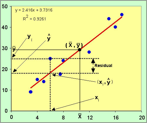
Now look at all of the arrows. They identify four points. The first to notice is xi, a data point chosen at random.
Follow the dashed vertical line up from xi until it gets to the regression line. That point is (xi, y-cap).
Y-cap is the symbol for the PREDICTED value of y, given a particular xi and the linear equation estimated by the least-squares procedure.
- the predicted value of yi for a given xi is gotten by substituting the value of xi into the linear equation (y = mx + b) and calculating yi
- So, all of the predicted values of y lie on the line. Note that the regression line has endpoints in the graph above. These are set by the largest and smallest x values.
- One can calculate a y value for any possible x value, whether or not that x value is in the data set or not
- if the x value is in the data set, then the y is one of the predicted y values
- if the x value is within the range of observed x values, then the y value has been interpolated
- if the x value is outside of the range of observed x values, then the y calculated from such an x value has been extrapolated
- extrapolated y values are subject to greater uncertainty than are interpolated y values
Remember - y-bar is the MEAN of the y's, y-cap is the PREDICTED VALUE for a particular yi.
If you follow the horizontal line over to the y-axis from (xi, y-cap), you come to y-cap on the axis.
If you go back to (xi, y-cap) and continue up the vertical line, you come to the data point, at (xi, yi) - the horizontal line over to the y-axis goes to yi.
The difference between yi and y-cap is the residual for yi.
Residuals
The line segment between (xi, y-cap) and (xi, yi) is the distance from the line to the data point. This distance is the RESIDUAL of yi, the difference between the predicted and observed values for this data point. Formally,
Residual = yi - y-cap.
Note that the vertical distance is not the shortest distance between the line and data point, but it is the correct one here because we are trying to use x to predict y, and the residual is the degree to which we have missed our mark.
Now that we have defined what a residual is, we can go back to the least-squares criterion.
I am sure that you have guessed by now that the criterion will minimize some aspect of the residuals.
We can't use just the residuals, as they are both positive and negative values, so some residuals would add to the total and some would reduce it. If the total of the residuals were used as the criterion, negative residuals would improve the fit!
So we need another term, the RESIDUAL SUM OF SQUARES:
This equation should be no surprise by now, but there is one thing you should look closely at. The second y term is y-cap, the predicted y, not y-hat, the average y.
Now we can simply state our Least-Squares Criterion
The "best" fitted line is the one that minimized the residual sum of squares.
Which slope and intercept represent the "least squares?" We have already calculated both. It can be shown (not here, but it's a simple derivation using the minimum of a quadratic equation with the coefficient of the squared term greater than 1, so that you have a minimum) that the b0 and b1 (formulae above) will define the line that results in the smallest possible residual sum of squares.
The residual SS gives us the ability to calculate the standard deviation of the residuals:
This formula means the same as any standard deviation: about 95% of all residuals will be within 2 standard deviations of the line.
Note the subscript of s. It is Y given X, meaning that x has been used to predict y.
Least-Squares is a parametric method, involving means and variances, and there are assumptions which must first be met before it is valid to apply the method.
Is this the only way to fit a line to the data?
No, but we will not go into non-parametric methods for fitting lines here.
PRACTICAL PITFALLS
Three other conditions often invalidate the use of regression.
CURVILINEARITY
This method assumes a linear relationship between x and y. Given that and the assumptions above, it does a good job. However, if the real relationship is a curve, not a straight line, then the method fails.
The blue points are not on a line, but you can still ask for a regression line (also in blue).
The black curve, generated by the polynomial equation yi = b0 + b1xi + b2xi2 + b3xi3, seems to be a better predictor of y.
OUTLIERS
These are data points that lie much farther from the regression line than the other data points, as the next to last green-square point (it is near the 16 on the x-axis).
Outliers have x values that lie within the extremes of the x values. It is the Y values that are unusually large or small.
Outliers can pull the line so that it is biased (compared to the line calculated without the outlier).
The green line (with the outlier included) looks as though it overestimates y when x is small and under estimates y when x is large.
Such systematic error is bias because you can predict which way the error will go.
Outliers might represent bad data points from experimental error or just bad observation.
INFLUENTIAL POINTS
Influential points are those that lie close to the line, but they are not near the other data points, as with the brown diamonds.
Influential points have x values that are far from the rest of the x values (it is the x that is unusually large or small)
An influential point has a greater contribution to the estimation of the regression line than do the other points, and so it might be an outlier, but it pulls the line near it so it looks like it isn't an outlier.
The one diamond set apart from the others looks like it is right on the line, but that's because it is influencing the line.
Look at the other diamonds. Does it seem obvious that the best line through them will pass close to the loner diamond? I think it would pass considerably below it.
Residual plots
Residuals can be plotted versus predicted y values.
Transformation of the Data
If the problem is that there is curvilinearity or that the standard deviation increases with x, then one of the transforms below may correct the problem by compressing the data's larger values:
- Logarithmic (natural or some other base)
- square root
- inverse
There are other transforms that are more involved (arcsine square root, logit, probit) that we will not cover here.
Inferences Concerning the Betas
A useful outcome of the parametric nature of the least-squares linear regression model is that one can use the b's to make statistical inferences.
If there is a relationship between two variables, then the slope of the regression line should be different from 0, a condition for which we can test.
If you were to take different samples of x and y, random error would mean that the estimates of the slope of the regression line would differ.
If this is so, then there is an expected distribution for the
1's drawn from independent samples from the same populations of x and y.
Note the substitution of
This is parallel to the situation in which we know that different samples from the same population will have different means, and that we can determine their distribution if we know the sample size (using the t-distribution).
The ![]() 1's are normally distributed, as are the means
(or difference between the means, etc.) so we need to know two things: the sample
size and the standard error.
1's are normally distributed, as are the means
(or difference between the means, etc.) so we need to know two things: the sample
size and the standard error.
As ever, the standard error is related to the standard deviation (in the numerator) but the denominator seems different. Instead of n, it is a sum of squares.
- This is because the effect of the denominator is to reduce the SE, which makes the calculated statistics smaller.
- When we were dealing with means, the larger the sample size, the smaller the SE.
- Here it is not all sample size. Look at the chart below.
- There are the same number of squares as circles.
- However the slope (b1) we estimate from the squares will be more accurate than will that estimated from the circles because the squares are spread out over a larger range.
So, the number of observations is important, but so is their dispersion.
- SS for x, which is what is in the denominator (with its square root - just as if it were simply the sample size) is a measure that will increase with both n (adding more terms) and with the spread of the x values (the difference between xi and x-bar is larger).
Confidence intervals and t-tests
Now that we have the standard error, we can use it to calculate both the confidence interval and ts , for a t-test.
CI = b1 ± taplha/2SEb1
Notice that the t-value we look up is half of the
-level (if we want a 0.05 alpha, then we look up 0.025) because we want a nondirectional t-value so we need to adjust from the book's table, which provides a directional probability.
To do the t-test, we simply calculate ts:
For the time being, ignore the last part of this expression. We know b1 and SEb1, so we can perform the t-test for the following hypotheses
![]()
H0 in English: There is no relationship between X and Y.
![]()
HA in English: There is a relationship between X and Y.
The degrees of freedom is = n - 2
This test assumes that there is a linear relationship and then asks if the slope can be distinguished from 0.
We can also test to see if the intercept is statistically different from 0, which can also be useful, but we will not cover this technique here.
Coefficient of Determination
We need to define a couple of terms before beginning this section:
Both are sums of squares and they look similar:
SS(total) is the SS of the y data points corrected for the mean of the y's (y-bar).
SS(regression) is the SS of the predicted y's (y-caps) corrected for the mean of the y's (so the difference here is between the predicted y and the mean y).
The relationship between the three SS for regression is:
SS(total) = SS(regression) + SS(residuals)
Think of it this way - the total variability is the sum of the variability explained by the regression, plus the leftover, unexplained variation (the residual variation - which is where the term residual comes from).
With this in mind, we can calculate the proportion of variation explained by the regression model.
This term is called the COEFFICIENT OF DETERMINATION and is represented by r2 (and better known as "r-square than as the coefficient!):
This term is often expressed as a percentage and it represents the proportion of total variation explained by the regression line. If all of the points lie on the line, then it is 100%, if any point lies off of the line (as all points do in the graphs above), then it will be somewhat less than 100%.
Look at the first graph above. The r2 is reported there for the fitted line. It is ~93%, which might be considered high by field biologists but might be greeted with less enthusiasm by laboratory researchers calibrating a standard curve for protein determination.
Although the book doesn't point this out, I feel that I should alert you to the fact that one can calculate r2 simply by squaring r, the correlation coefficient discussed in the next section.
One thing that r2 does not tell you is anything about the actual relationship between x and y. You know how good the fit is, but not what is being fitted.
This can, of course, be gotten from the regression equation.
If the slope is positive, then as x increases, so does y. If it is negative, then as x increases, y decreases.
Correlation coefficient
Sometimes, the exact relationship is not of interest, only the degree of association between two variables.
This relationship (=association) is called the correlation between x and y. The strength of the correlation and whether it is negative or positive is given by a single statistic, r, the CORRELATION COEFFICIENT (also known as the Pearson Product Moment Correlation Coefficient):
It is the ratio of the COVARIATION between x and y (corrected for their respective means) to the total variation in both x and y (once again corrected for their respective means)
Covariation means just what the term implies - when (x - x-bar) is large (in absolute terms) and negative, is (y - y-bar) also large and negative? When x - x-bar is small and positive, is y - y-bar also small and positive?
- If (x - x-bar) is positive, and (y - y-bar) is positive, then the resulting term is positive
- If(x - x-bar) is negative, and (y - y-bar) is negative, then the resulting term is positive
- If (x - x-bar) is positive, and (y - y-bar) is negative, then the resulting term is negative
- If (x - x-bar) is negative, and (y - y-bar) is positive, then the resulting term is negative
So you can see, that if x and y always match signs, the numerator will turn out to be positive, If they don't match, the numerator will be negative.
The denominator is always positive due to the squaring, so whether or not r is positive or negative depends on the degree of matching in the numerator.
A negative r indicates an inverse relationship (as x gets large, y gets large)
r = 0 indicates no relationship between x and y
A negative r indicates an inverse relationship (as x gets large, y gets small)
Testing the significance of r
Does r differ from 0? This will be true only if the slope of the regression line is 0 but we often get r without knowing the regression line.
But - look back at the expression for calculating
ts to do a t-test for ![]() - the last part of it has only r and r2 in it. So, without
knowing b, we can reject or accept the following hypotheses:
- the last part of it has only r and r2 in it. So, without
knowing b, we can reject or accept the following hypotheses:
H0: r = 0
H0 in English: There is no relationship between X and Y.
![]()
HA in English: There is a relationship between X and Y.
The degrees of freedom is = n - 2
To
do the test, calculate ts, compare
it to the t-value associated with the chosen ![]() -value,
and reject the null if ts is larger than, accept the null if it
is smaller. You are testing the slope's difference from 0, which is
equivalent to the null and alternative hypotheses above.
-value,
and reject the null if ts is larger than, accept the null if it
is smaller. You are testing the slope's difference from 0, which is
equivalent to the null and alternative hypotheses above.
Last updated December 1, 2011