Confidence Intervals

Chapter 6 (4^th edition) or Chapter 6 (3^rd edition,except sections on proportions) and part of Chapter 7 (3^rd edition, first sections on confidence interval of the difference between means)

Email me

Back to:

Unit Organization:

• Statistical Estimation
• Standard Error
• Confidence Interval for the true mean
• How large a sample size?
• Validity of Confidence Intervals
• Independent Samples and the difference between means
• Standard Error of the Difference Between Means
• Confidence Interval for the Difference Between Means

Problems:

Problems for homework

• 3rd edition: 6.3, 6.7, 6.10, 6.25, 6.29, 6.32, 6.34, 7.4, 7.5, 7.19, 6.52, 6.58
• 4th edition: 6.2.3, 6.2.7, 6.3.3, 6.3.19, 6.4.4, 6.5.2, 6.5.4, 6.6.3, 6.6.4, 6.7.11, 6.S.2, 6.S.8

Suggested Problems

• 6.1, 6.2, 6.12, 6.14, 6.16, 6.18, 6.27, 6.31, 6.39, 6.43, 7.1, 7.2, 7.11, 7.17, 7.18, any from the section of problems at the chapter's end
• 4th edition: 6.2.1, 6.2.2, 6.3.5, 6.3.8, 6.3.10, 6.3.12, 6.4.1, 6.5.1, 6.6.1, 6.6.2, 6.7.2, 6.7.9, 6.7.10, any from the section of problems at the chapter's end

Statistical Estimation

This is the reason for doing statistics in the first place.

Statistical estimation has two components

• estimation of some population parameter (mean, st. dev., shape of the distribution, etc.)
• determination of the precision of the estimate (how likely is it to be correct?)

In this lecture, we will learn how to construct confidence intervals, which depend on us knowing two things:

• an estimate of the true mean
• an estimate of the spread of the data about the true mean

As discussed before, the best estimate of the true mean is a sample mean (or, better, a mean of sample means)

this leaves us with the problem of estimating the true standard deviation (it's not exactly s)

Standard Error of the mean

• First, let's recall what the standard deviation is:
  • a measure of the dispersion (=spread) of the data around the mean, variation causes the data points to differ, not error
  • when there are lots of big and small values but few in the middle, the st .dev. is larger than when most of the data is near the mean
• The standard deviation of sample means is caused by sampling and measurement ERROR, not variation (by our definitions) and so should really be called "error" not "deviation" but we will follow standard usage
  • The standard deviation of sample means is likely to be smaller than the standard deviation estimated from a single sample or the true population standard deviation
    • When means are calculated from samples drawn randomly from a population, they will most often be closer to the true mean than will a single data point drawn from the population at random
    • Thus, a standard deviation calculated from 10 means will be smaller than a standard deviation calculated from 10 values drawn at random from the population
• Thus, to calculate the standard error of means, we need a formulation that will guarantee that it is smaller than the population standard deviation ()
• There is a second consideration and that is that samples are not all equally good
  • Means calculated from large samples are more likely to be nearer the true mean () than those calculated from small samples.
  • If this is so, then a standard deviation calculated from small sample means (which are clustered less tightly about the true mean) should be larger than a standard deviation calculated from large means (which are clustered more tightly about the true mean)
• So, taking both considerations into effect, we use this equation:

• Note that we use the square root of the sample size (remember that  is a square root also)

• A practical problem is embedded in the above definition of the standard error of sample means.
  • To calculate the standard deviation of the means, we needed the standard deviation of the population
  • This is not usually something we know, so we need a fix, a way to estimate this from a single sample
• So, what can we use to estimate sigma, ()?
  • If we get something to estimate sigma with that we can actually measure, then we can use it to find the probability of a sample mean being close to the actual mean ()
    • The most obvious estimate, and the one we will use is s, the standard deviation of the sample, which we will substitute into the formula for the standard deviation of the sample means

• We call the standard error (SE) of the mean, not the standard deviation of the mean because it is a measure of the error in the sample mean, not a measure of the variation among data points.

Difference between SE and SD

• Standard deviation of the sample - refers to how the individual data points are distributed with respect to the mean, it is a measure of data dispersion.
  • Remember how it is computed (as the square root of the average [corrected for degrees of freedom] of the squared deviations of the data points from the mean [remember we square as a means of making all of the deviations positive])
• Standard Error of the mean - refers to the probability that sample means, not individual data points, differ from the true population mean
  • The book states the same thing with different words. The book defines the SE as a measure of uncertainty due to sampling (random) error in how good a sample mean is as a measure of the true mean
  • A larger SE means there is more uncertainty in using the sample mean as an estimator of the true (population) mean
  • Remember that SE is related to s, but that it is always smaller than s
    • The divisor means that larger samples have a smaller SE, that is, that they are expected to be closer to the true mean than are sample means from smaller samples

Confidence Interval for the True Mean

A confidence interval is a range of values between which we believe the value of interest to lie

• for us , the mean of the population, is the value of interest

The size of the range depends on two things

• how sure (confident) we want to be
  • if we want to me more sure, then we must have a larger range
    • you can be somewhat sure that the true mean of the student age at TSU is between 20 and 30
    • you can be totally sure that the true mean of the student age at TSU is between 1 and 100
• how much random variation there is the original population
  • If we knew , the population standard error, we could get the range for , the sample mean, given that the population is normally distributed
    • if you want to know how big a confidence interval you need to be 75% sure that the mean is in the value you have to find the z values that have 75% of the area under the normal curve between them (see below, to see that these values are about -1.03 and 1.03)

Then one would find X, the actual numbers, from the z values (remember how you calculate a z) as done below

The confidence interval when sigma is known:

Start with the proposition that the probability of Z being between -1.03 and 1.03 is 75%

Pr{ -1.03 < Z < 1.03} = 0.75

Substitute the formula for calculating Z based on the sample mean (because it has and in it, and we want to know how one relates to the other)

Pr{-1.03 < < 1.03} = 0.75

Now do some simple algebra to find out where should lie

• first, multiply by the denominator, , to eliminate it from the middle term and then subtract to remove it from the middle term, last multiply by -1 )
  • Pr{-1.03*    <   -    <   1.03*} = 0.75
• subtract  from all 3 terms and then multiply by -1 to turn a negative into a positive (with the appropriate changes in the direction of the inequality signs) and you get
  • Pr{-1.03* -   <  - < 1.03* - } = 0.75
  • Pr{ - 1.03*   <    <  + 1.03*} = 0.75
• This last expression is a confidence interval.
  • It says that there is a 75% chance of the true mean being between the sample mean minus a term (based on a z value and the standard error of sample means) and the sample mean plus the same term.

What if we do not know the value of the standard deviation of the population?

We have done it, we have found out where the true mean is with a confidence level of 75% but there is a fly in the ointment, a bit of unfinished business

• How can we find unless we know ?
  • We need an estimator of and we will turn to the same place as before, the SE of the mean (which was discussed above)
• There is a second problem, because the normal was calculated with , not with SE or S
  • It turns out that the distribution of means follows a curve called Student's t, which is similar to the normal
    • it is symmetric with a single mode, just like the normal
    • it has a larger standard deviation term than does the normal
    • the difference between the t distribution and the normal is dependent on the sample size, such that smaller sample sized are less like the normal and larger are more similar
    • when sample size is infinitely large, the t and the normal distributions are identical

Calculating a confidence interval using the t-distribution

We can re-write the last equation for a confidence interval now

Pr{-t_0.75*SE_x ¾ ¾ +t_0.75*SE_x} = 0.75

so we need to calculate

± t_0.75*SE_x

• We know how to do the sample mean and SE (from above), but what is t?
  • t refers to the student's-t distribution.  It is a platykurtic (flattened) version of the normal distribution.  There is more than one student's-t distribution.  In fact, each sample size produces a unique t-distribution.
    • The shape of the distribution changes with n, the sample size.  As n gets larger, the student's-t distribution becomes more and more similar to the normal (in fact, when n is infinitely large, they are the same.
  • In the figure below, the normal curve is in pink and is the curve with the highest peak that falls most steeply.  Compare it with the student-t curve for 1 degree of freedom (k is the degrees of freedom, which depends on the sample size - see below), which is black. The x-axis units are standard deviations and the y-axis is probability.

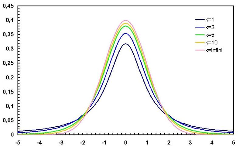
diagram from Wikipedia, Student's t Distribution entry, used here under GNU license

• The peak of the student's-t distribution (black) is lower than the normal (pink) and the tails on either side for the student's t distribution are higher than for the normal distribution.
  • This means that, if I compare the areas under the curves that are less than -2 sd, then the area will be larger for the student-t distribution than for the normal.
  • Consider this:  Which curve has more area within ± 1 sd of the mean (= 0 here).  Since there is more area out in the tails for the student's-t distribution, then there must be less in the center,  so it is the normal with more area (= greater probability) within a standard deviation of the mean.
  • This makes sense.  A sample provides an estimate of the population.  Estimates are not as accurate and so a curve based on estimates should have more "spread."  As the size of the sample increases, the estimate gets better and better, which happens here because the student's-t distribution becomes more like the normal  is n increases.

• We can look the cumulative areas (probabilities) up in table 4, where the table body is the upper tail probability of the t-distribution and the rows an columns depend on the degrees of freedom and the critical value you want to use
  • Degrees of freedom are n-1 when only one parameter is being estimated (we are trying to estimate only )
• The table lists only the upper tail, and we are concerned about being both too small as well as too large, so we need to divide the area of the tails (= 1 - confidence level) in half to look it up
  • if you want a confidence of 95%, then (1 - confidence level) = (1 - 0.95) = 0.05 but you have to look up 0.025, not 0.05

How Large a Sample Size

This is an important question to ask when designing experiments.

• If you will be using statistics to evaluate the results, then you don't want
  • to have too few data points to show a difference between experimental and controls
  • to have more data points than is necessary to show a difference between experimental and controls
• The first instance can be a disaster and the second may be an inconvenience (doing more than needs to be done) or can mean that you get fewer experiments done because you are wasting effort

We will use the formula for the standard error of the mean to estimate n (see above for this formula)

• You can't do this without some sort of guessing, but the guessing should make use of prior knowledge and your expertise.
• Consider what you want the ± portion of the confidence interval to be (see example below)
  • You are measuring the concentration of a protein, and you think that the experimental cells might have as much as 20% more than the control cells. You will have to set up a series of flasks in which to rear cells and will measure the concentration of the protein in each flask. How many flasks do you need to set up?
  • You know that the control cells produce (from the literature or from previous work) about 25 picograms per microliter of protein with a standard deviation of 7 picograms per microliter.
  • You want to be 95% confident that your estimate of the concentrations will be within 5 picograms per microliter of the true mean
    • The 95% is an arbitrary choice, but it means that you have only a 1 in 20 chance of being wrong
    • You chose the 5 value because you expect the experimental to only be about 5 microliters above the controls (20% of 25, the known mean).  At this stage, this must be a guess based on the experimenter's experience or on the results of similar experiments.
  • So you want the ± portion of the confidence interval to be no larger than 5
    • the ± portion is t_0.025*SE_x,
      • t has the subscript of 0.025 because you want to be 95% confident, so the critical value is 5% (1-0.95) and this is divided in half because the table has only the upper tail probability (=area under the curve), and you are concerned about both the upper and the lower tails (missing by being too large or too small an estimate)
    • from the table, t_0.025=~2 (you don't know the degrees of freedom yet, but look at table 4 in the 0.025 column, and the values drop to about 2 very quickly, so 2 is a reasonable estimate)
  • So, we can find N now because we have all the information we need
    • 5 = t_0.025*SE_x,
    • 5 = 2 * S, and SE_x = S/sqrt(n)
    • 5 = 2 * 7 /sqrt(n)
    • sqrt(n) = 14/5 = 2.8
    • n = 2.8^2 = 7.84, so you need about 8 flasks to make an estimate accurate enough for your purposes

Validity of Confidence Intervals

First, the SE_x must be a valid estimate of

• The sample must be chosen from the population in a random manner, such that each member of the population has an equal chance of being in the sample.
• The population size (N) must be large when compared with the sample size (n).
• The observations must be independent
  • one observation (x) must not influence the size of other observations (x's)
  • consider the removal of a sample and then not replacing the sample
    • you are measuring an enzyme in the gut of rats
    • you have 5 rats and you take out the intestine and cut it into six pieces. Enzyme concentration is measured in each piece of gut
    • How many observations do you have? You have 30 (5 rats times 6 pieces per rat)
    • How many independent observations do you have? You have only 5 because the six from the same rat might all be influenced by the individual characteristics of the rat, and you are not interested in that rat per se, but in all rats

The confidence interval is valid if

• the SE_x is valid
• the population from which the sample is drawn is normally distributed

this condition is strict if you want the CI to be valid for small sample sizes

this condition can be relaxed if the sample size is large, in which case the population distribution is of no consequence (remember the central limit theorem)

Independent Samples and the Difference Between Means

• We often want to compare two different populations.
  • Control versus Experimental
  • Male versus Female
  • Old versus New
• We do this by drawing random samples from each population and comparing the samples.
• Populations must not overlap, so that the samples drawn are INDEPENDENT of one another.
• Any population parameters may be compared, but we will, once again, concentrate on the mean as the best way to compare populations (this is not always true).
  • To do this, we will speak about a composite statistic (or parameter), called the DIFFERENCE BETWEEN MEANS (the subscrips 1 and 2 are used to identify the different populations or samples)
    • For populations this is: ₁ - ₂
    • For samples this is: ₁ ^- ₂

Standard Error of the Difference Between Means

We will use the standard error of the mean, SE_xbar, to get the Standard Error of the difference between means (= SE_{(x1 - x2)})

• There are two ways to approach this.
  • One pools the variance of each sample to get an overall variance and then calculates the standard error from this pooled variance
  • The second is called the unpooled SE and it uses SE from both samples
    • If the 2 sample standard deviations are equal or if the sample sizes are equal, then the pooled and unpooled SE's are equal
• When the sample sizes are unequal, then we must choose which to use
  • If the standard deviations of the POPULATIONS are EQUAL, then the pooled is the correct choice
    • However, the unpooled will be close to the pooled SE
  • If the standard deviations of the POPULATIONS are UNEQUAL, then the unpooled is the correct choice
  • The book recommends that the unpooled be the only choice, because:
    • the potential problems caused by choosing the unpooled when the pooled is the correct choice are small because the unpooled estimate and pooled estimates are usually about the same size in this case
    • the potential problems caused by choosing the pooled when the unpooled is correct choice can be very serious, leading to false conclusions
• So we will only work with the unpooled SE (the pooled SE formula is in the book)

or

This second form is the same as the first if you substitute for SE using the definition of SE in the previous chapter.

Confidence Interval for the Difference Between Means

Once you have calculated the standard error of the difference, this is just an adaptation of the CI formula above:

• Notice that I have chosen 95% as the confidence level. It can be something else, but then the t-value would have to be adjusted
• Notice also that the CI is for the difference between parameters (population means) and is calculated from sample statistics

In order to look up the right t value, you need to know the degrees of freedom, which represents a bit of calculating:

SE₁ and SE₂ are the sample errors (the sample standard deviation divided by the square root of the sample size)

• This formula = n₁+n₂-2 if SE₁ = SE₂ and n₁ = n₂ and approaches n_min - 1, where n_min is the smaller of n₁ and n₂, as sample sizes and standard errors become less and less equal
• The formula above is the most accurate means of determining the degrees of freedom.  However, you could use either n₁+n₂-2 or n_min - 1 as long as you are aware of the cost
  •  n₁+n₂-2 gives a confidence interval somewhat smaller than it should be if the SE's and n's are not equal
  • n_min - 1 gives a confidence interval somewhat larger than it should be unless the SE's or the n's differ greatly

This test is valid when:

• each sample is a random sample of independent observations
• the populations are normally distributed if small populations (relaxed assumption for large populations due to Central Limit Theorem)

Last updated October 5, 2011