|
 |
BIOL 3110
Biostatistics
Phil Ganter
301 Harned Hall
963-5782 |
Comparison of Paired Samples
Chapter 8 (4th ed.)
or 9 (3rd ed.)
Email me
Back
to:
Unit Organization
Problems
- Problems
for homework
- 3rd
edition - 9.1,
9.2,
9.14,
9.19,
9.28,
9.30,
9.38,
9.39,
9.40
- 4th
edition - 8.2.1, 8.2.2, 8.4.1, 8.4.5, 8.5.1, 8.5.3, 8.S.1,
8.S.2, 8.S.3
- Suggested
Problems
- 3rd
edition or
4th edition - There
aren't that many problems in this chapter, so all of
the problems not assigned above are recommended as practice
Paired-Sample
t-test
What is meant by Paired?
Whenever two observations are, for some reason,
linked such that you suspect that they should be more similar to one another
than to the rest of the data, then you have paired observations. A Paired Sample is a set of paired observations.
- Paired observations might be before and after
samples from the same individual or right side-left side observations from
the same individual.
- It is not the before-after that makes them
paired, but the fact that they came from the same individual.
- Paired observations might be from different
individuals that have been matched for some set of characteristics (similar
size, age, etc.).
What is the Paired Sample t-Test?
- The paired test statistic is the difference between
the paired observations, which is symbolized by d (for difference).
 is average difference. Note that
  has the same value as the difference between the means
of the two samples (ave. after minus ave. before, etc.).
- The mean of the differences is the same as the
difference between the means (
 =
=  1 -
1 -  2 ).
2 ).
- One
can also calculate the standard deviation of d, sd.
in the normal way using d (the differences) as the observations.
- The sample size (n) is simply the number of
paired observations.
- The test asks the question: Is
there a difference between the size of the paired observations?
H0 :  = 0
= 0
Ha : 
 0
(non directional)
Standard Error = SEdiff = sdiff /sqrt(n)
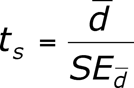
- The t-value you calculate is like you have done
before. It is the ratio of a statistic divided by the standard error.

There are n - 1 degrees of freedom.
- p-hat = Pr{ts} = The probability of
being wrong (committing a type I error) if one rejects H0. As
before, one looks up p-hat in the t-table using the value of ts and
n-1 degrees of freedom.
- Evaluation of Pr{ts} is like any
other t-test. If p-hat is smaller than the pre-selected
 -value, then the risk of making a mistake is less than
the acceptable risk, so you go ahead and reject the null hypothesis. If
it is larger, then the risk is greater than you said you would accept.
CONFIDENCE INTERVAL for
a paired design
- The confidence interval is close to that for a
difference between means. The difference lies only in the smaller SE expected
for the paired design.
 ± ta,df(SEd)
- The
t-value depends on the chosen alpha value and the degrees of freedom, which
are the same as for the t-test (n-1)
- Under
what assumptions is it fair to use a paired design?
- First, you must suspect that the pairing are reasonable.
Then the assumptions are the same as for the t-test in general.
- d must be calculated from a random sample.
- the d's must be distributed normally when the
sample size is small. This assumption is relaxed as the sample size gets
large due to the effect of the central limit theorem.
Paired Experimental Designs
- Why do we do a paired t-test
rather than a regular comparison of sample means?
- There are two reasons for using a paired design:
reduction of bias and/or increased precision. Both reasons may be true at
once.
- The difference in the outcome usually lies in the
standard error of d being smaller than the standard error of the difference
between the means (although the degrees of freedom is usually greater in
the second case).
- This area can be best explained with two examples.
- Reduction of bias.
- Suppose that you are conducting an experiment in
which plant size is being compared for plants treated with a pesticide versus
control plants without treatment. You are going to grow the plants in pots
on a table in a room with a large window on one side. The 24 pots will fill
the table in eight rows of three pots, with the side of the table with eight
pots parallel to the window. You suspect that the plants in pots on the side
of the table away from the window will get less sunlight in general and will
be smaller. Thus, you suspect that bias is part of the design because there
is a systematic difference in growth due to pot position.
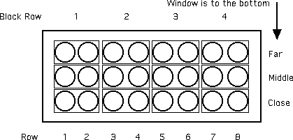
- A randomized blocks design is a way of reducing
bias. But how to block? I suggest that you use small blocks: pairs
of pots. Each pair is two adjacent pots in the same row of eight, so that
each pot gets the same amount of sunlight. See the diagram:

- Each pair of circles in a small rectangle represents
a block. Treatment or control is assigned randomly to each pot. The idea
here is that there will be little difference in sunlight along a row and
you will be allocating randomly within the block. Now you have 12 pairs
of observations (linked by being in the same block) and can used a paired
design. Look at the results (cooked up by me) and you will see that
there was bias in the design (notice that the far plants are much smaller,
as predicted).
| Position |
Block |
Treated
(ounces)
|
Control
(ounces)
|
d |
| Close |
1 |
57 |
52 |
5 |
| Close |
2 |
56 |
55 |
1 |
| Close |
3 |
57 |
53 |
4 |
| Close |
4 |
59 |
56 |
3 |
| Middle |
5 |
37 |
32 |
5 |
| Middle |
6 |
36 |
35 |
1 |
| Middle |
7 |
37 |
33 |
4 |
| Middle |
8 |
39 |
36 |
3 |
| Far |
9 |
17 |
12 |
5 |
| Far |
10 |
16 |
15 |
1 |
| Far |
11 |
18 |
13 |
5 |
| Far |
12 |
19 |
16 |
3 |
| |
| |
mean |
37.33 |
34.00 |
3.33 |
| St Dev |
16.99 |
17.14 |
1.61 |
| n |
12 |
12 |
12 |
| SE |
4.90 |
4.95 |
0.47 |
| |
| difference
in means |
3.33 |
|
| unpooled
SE |
2.01 |
| |
|
|
| ts
for paired comparison |
7.15 |
| ts
for unpaired comparison |
1.66 |
| |
|
|
| d.f.
for paired comparison |
11 |
| d.f.
for unpaired comparison |
22 |
| |
|
|
| p-value
for paired |
0.00002 |
| p-value
for unpaired |
0.11 |
- Notice that I have calculated p-hat for two different
scenarios: a paired design and an unpaired design.
- The standard error of
 (0.47) is much smaller than the unpooled SE
for the difference between means (2.01) so the ts-value for
  is much larger because the SE's are different while
the numerators are not.
- Thus, p-hat is much less for the paired design
than for the unpaired design (remember that this is an extreme case with
cooked data).
Increase in Precision
Here, we will just give some numbers for an undescribed
experiment with two samples, each with six replicate samples. Assume that
the six can be paired and look at the difference in the analysis depending
on whether or not the observations are paired.
| |
Treated |
Control |
d |
| 36 |
29 |
7 |
| 57 |
43 |
14 |
| 99 |
83 |
16 |
| 23 |
11 |
12 |
| 45 |
32 |
13 |
| 71 |
64 |
7 |
| |
| mean |
55.17 |
43.67 |
11.50 |
| St Dev |
27.13 |
26.00 |
3.73 |
| n |
6 |
6 |
6 |
| SE |
11.08 |
10.61 |
1.52 |
| |
| difference in
means |
11.50 |
|
| unpooled SE |
6.26 |
|
| |
| ts for paired
comparison |
|
7.56 |
| ts for unpaired
comparison |
1.84 |
|
| |
| d.f. for paired
comparison |
|
5 |
| d.f. for unpaired
comparison |
10 |
|
| |
| p-value for paired |
|
< 0.001 |
| p-value for unpaired |
> 0.10 |
|
In this case, just look at the two samples and
notice that in both there is a lot of variation between observations within
each sample. This makes the unpooled standard error large. However, the differences
(d's) show much less variation and so their standard error is much smaller.
This leads to very different p-hat values.
A Nonparametric Approach: the Sign Test
- This test is useful when sample size is small and
there are real doubts about whether or not a t-test can be used.
- It is based on the sign of the difference between
paired observations.
- Let's restate the null and alternative hypotheses
so that we are clear:
H0 :  = 0
= 0
HA : 
 0
0
- If H0 is true, then the error between
the observations is random. If this is so, then there should be an equal
chance of getting a positive difference or a negative difference. That
is, we expect half of the signs to be + and half to be -.
- The signs test is based on this assumption and
the binomial distribution.
- If we have n pairs, then half of the pairs
should yield + d's and half should yield - d's.
- The probability (
 ) of getting a + or a - in each case
is 0.5.
- If we actually get j positives, what is
the probability of that?
- This is a binomial, with
 = 0.5 and we are asking about
j successes in n trials
- Remember
that we are dealing with the probability in the tail of the distribution,
so we need to include not just the probability of getting j successes but
also the probability of getting all of the successes in the tail. This
means you should draw the tails out and figure out which probabilities
you need to calculate.
- What to do with tied pairs,
so that d = 0.
- Ignore them. Remove them from the dataset and
proceed as above.
- Evaluation
- In order to make this into a test that is equivalent
to the t-test, we have to have a criterion for accepting or rejecting the
null.
- We will use the same one but it is not exactly
straight forward. First, select an
 -value.
- Nondirectional
- Suppose that there are 20 d's and we get 17
-'s and 3+'s.
- If the sum of the probability of getting 17
or more minuses (notice that this includes J = 17, 18, 19, and 20) plus
the probability of getting 3 or fewer minuses (j = 3, 2, 1 or 0) is less
than
 , then we will reject H0.
- Why
17 or more minuses? Because the tail of the distrubution includes all
of these values of j!
- Why
3 or fewer minuses? Because, for a nondirectional test, we need both
tails, and 3 to 0 is the lower tail that corresponds to 17 to 20, the
upper tail!
- Directional
- Using the example above, we first must decide
which direction is of interest. Lets look at the possible HA's
- HA :
 > 0
> 0
- Since there are 17 -'s, then the average d
must be a negative number, which means our alternative can't be true, so
nothing more need be done.
- HA :
 < 0
< 0
- If the sum of the probability of getting 17
or more -'s is less than
 then we reject H0.
- You can also use table 7 in the book, but it
is not as exact as the procedure above.
- When can you use the signs
test?
- There are few assumptions.
- The
sample must be a random sample and each d value must be independent
of other d values
- If
it is reasonable to assume that the d's are as likely to be positive
as negative, then the test is valid.
- No particular distribution is assumed.
- However, you should realize that much information
is in the data that is not being used for this test, which makes it's power
lower than that of a parametric test like the t- test.
- The lack of power (as defined in an earlier
lecture) means that you are more likely to accept H0 when it
is false.
A Nonparametric Approach: the Wilcoxson Signed-Rank
Test
- This uses a bit more information than does the
signs test, so it is a bit more powerful.
- To
do this test, rank the d's (the differences, not the original data!)
from smallest to largest (based on their absolute value).
- Restore
the + and - signs to the ranks.
- Add the negative ranks and take their absolute
value.
- Add the positive ranks.
- The test statistic (Ws)is whichever is the larger of the two sums
above.
- Evaluation
- The null and alternative hypotheses are as for
the signs or t-test.
- First,
select an
 -value. After calculating Ws, look up the
 -value in the table at the back of the book
- Nondirectional
- Reject
the null if Ws is
larger than the Wilcoxson Signed Rank Test table entry
for n and the two-way
 .
.
- Directional
- First must decide which direction is of interest.
Lets look at the possible HA's
- HA :
 > 0
> 0
- If Ws is the summed positive ranks,
then it makes sense to proceed with the test. If Ws is the summed
negative ranks, then d was usually negative and it makes no sense to perform
the test.
- Reject
the null if Ws is
larger than the Wilcoxson Signed Rank Test table
entry for n and the one-way
 .
.
- HA :
 < 0
< 0
- If Ws is the summed negative ranks,
then it makes sense to proceed with the test. If Ws is the summed
positive ranks, then d was usually positive and it makes no sense to perform
the test.
- Reject
the null if Ws is larger
than the Wilcoxson Signed Rank Test table entry for n and
the one-way
 .
.
- When can
you use the Wilcoxson Signed-Ranks test?
- The
sample must be a random sample and each d value must be independent
of other d values
- If it is reasonable to assume that the d's
are as likely to be positive as negative, then the test is valid.
- The
d's (differences) need not be normally distributed but their distribution
must be symmetric. This is best assessed by a histogram of the
differences.
Last updated October 27, 2011
![]() = 0
= 0![]()
![]() 0
(non directional)
0
(non directional)
![]() ± ta,df(SEd)
± ta,df(SEd)
![]() = 0
= 0![]()
![]() 0
0