 |
BIOL 3110
Biostatistics
Phil Ganter
301 Harned Hall
963-5782 |
| Endemic flower from the Serro do Cipo
Mts. in Brazil |
Categorical Data 1
Chapter 9 (4th ed.)
or 5.2, 6.6, and 10.1 (3rd ed.)
Email me
Unit
Organization:
Problems:
- Problems
for homework
- 3rd
edition - 5.1,
5.4 (modified), 5.5 (modified), 6.36, 6.40, 10.3,
10.6
- 4th edition
- 9.1.1, 9.1.4, 9.1.5, 9.2.1, 9.2.5, 9.4.3, 9.4.6,
- Suggested
Problems
- 3rd edition
- Try additional problems in the section where the required problems
are found.
- 4th
edition - There aren't that many problems in this chapter, so all
of the remaining
problems
are recommended.
Sampling Distribution from Categorical Data
We
have discussed the sampling distribution of the mean in the previous chapters. When
we measure some attribute of an experimental or observational unit, we can
use a mean to describe the central tendency of the measurements.
- Sample
mean (
 ) is the statistic we used to infer
something about the true population means (
 , the parameter)
- Sample
means are distributed
normally if either the population from which they are drawn is distributed
normally
or
if the
samples
are large
(Central
Limit
Theorem)
However,
not all data can be described by the mean. Categorical data are described as proportions of the total sample, i.e. frequencies.
So,
what then is the distribution of sample proportions?
- First,
lets define the parameter and statistic for proportional data The
true population proportion is p in the book. This is a bit of a
departure and I wonder why they have not stuck to the older practice
of using a Greek
letter for
the true proportion of the category in the population.
- We
will stick to the textbooks's usage and call the true population proportion
p (the parameter)
and the proportion of of a category in a sample from that population is

- We
normally estimate the proportion of successes (=
 , p-hat) as the number of successes divided by the number
of trials, so if there were 3 successes out of 10 trials then:
 =
3/10 = 0.30
- However,
a correction,
called the Wilson-adjustment, is necessary
- To
distinguish between the adjusted and non-adjusted calculation of the
proportion of successes, we will designate the adjusted proportion as
 (=p-tilde)
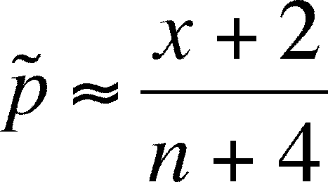
which is calculated from as:
- Now
(using the example above) it's
 =
(3+2)/(10+4) = 5/14 = 0.357
- Why use this adjustment? It is an outcome
of the fact that proportions are bounded (p can't be smaller than 0 nor
larger than 1)
- The probability distribution of
 "piles up"
at the boundaries", i.e. the distribution of a particular
 is not symmetrical
except for one special case
- Consider three proportions, p = 0.05,
0.50, or 0.90.
- The asymmetry means that
the chance that
 will be between 0 and 0.05 is greater than the chance
that it will be between 0.05 and 0.10 - a point just as far from
0.05 as 0 is
- At the upper end, the chance that
 will
be between 0.90 and 1.00 is greater than the chance of it being
between 0.80 and 0.90, once again a point as far from 0.90 as
1.00 is
- The special, symmetrical case is the
third proportion mentioned above. When p = 0.50, the distribution
is symmetric
- Thus, we need an adjustment that takes
this asymmetry into account and the Wilson adjustment will always
move
 closer
to 0.05 than
  is.
is.
- Note
that as n and x get larger,
 approaches
the value of
  , which is reasonable as less of a correction is needed
So,
what is the distribution of  (or
(or  ),
given that the true proportion is p? Once
again, a metaexperiment is where to begin.
- Each
experiment involves a series of observations, each one with a set number
of possible outcomes (categories)
so the data is summarized as the frequency (how many) or the proportion of observations
that belong
in
each
category.
- The
results of an experiment are the frequency of each category and
may be expressed as proportions (which, according to our frequency
definition of probability, are also estimates of the probabilities
of the outcomes)
- Each
experiment produces an estimate of the true probability (p),
which is p-hat (
 )
)
- Repeat the experiment time and time again, each time producing another

- The
distribution of the
 s
is graphed as a histogram with
  on
the x-axis and the frequency of each
  as
the y-axis. The question before us is this: what shape will that histogram take? Can
we predict the distribution of the
  s?
s?
- We can. It is the binomial, a distribution we already know. To
see why the binomial is appropriate, lets look at a simple example
- We need an experiment with categorical
data. How about
sampling a population and assessing the genotype of individuals
at a single locus with only two possible alleles (let's keep it
simple)? Thus, we have three categories (HH, Hh, and hh)
and a proportion of the total number of individuals in each category
- Now, consider any of the genotypes. How
would we expect the sample proportions, the
 s, to be distributed?
- If there are n individuals in the sample,
 might be any one of n + 1 discrete values (the binomial
distribution is a discrete distribution): 0, 1/n, 2/n, 3/n,
up to n/n. Each one of these proportions is one of the
possible outcomes of the sample (the experiment) and these are
the only
possible outcomes.
- Before, the x-axis for a graph of
the binomial distribution was J, the number of successes, and
the range
was from 0 successes to n successes
- We can calculate the probability of
each of the possible outcomes, the possible values for
 if we know the p (the actual proportion of that genotype in the
population) because the experiment (our sample) gives us
n and each possible outcome will give us a j (the j's will
be the numerator from each possible outcome -- remember,
to
calculate
the binomial, we need p, n and j).
- Note that the binomial applies, even
though there are more than two categories of outcomes.
- When
considering any one category, an individual that belongs
in that category is a success and individuals belonging to
all the other categories can be lumped together as failures,
which makes the outcome either a failure or a success, hence
the binomial distribution can be used
- If
 is the estimate of
  ,
then how close can we expect
  to be to
  ?
How good is the estimate? This depends on the number of events in
each experiment (n)
- Note that only certain estimates of
p are possible.
- If n = 4, then we can estimate p as 0,
0.25. 0.5, 0.75, and 1.0 only
- If n = 5, then we can estimate p as 0,
0.2. 0.4, 0.6, 0.8, and 1.0 only
- if
 =
0.3 and n = 4, then we can get a
  of either 0.25 or 0.5,
but not 0.3. The sampling distribution if
  will peak at 0.25 (because
it is closest to
  ).
).
So, the most probable
p-hat turns out to be p, the true probability of success
Confidence Interval for a population proportion
The
confidence interval for p will need an estimate of the standard error of
p and an estimate of p, both of which are presented below and an assumption
about t.
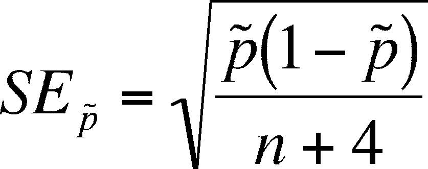
- The
last portion is what to do about the probability distribution of the
proportion. We
will use the normal, not the t-distribution., so we will estimate the
95 % interval using 1.96 (from the normal) but you can substitute the appropriate
z-value if you want to use a different level of confidence

 Test for Goodness-of-Fit
A goodness-of-fit test tests whether or not the
data conform to some prior expectation for the data.
- The prior expectation can come from a model
or from previous experience or can be a null expectation.
- As an example of a model that we all know, Hardy-Weinberg
predicts that one should find p2 of AA, 2pq of Aa, and
q2 aa individuals
in a population, if p and q are the frequencies of A and a, respectively.
- One might ask if the actual frequency
of genotypes from a population agree with Hardy-Weinberg expectations.
- This is a good case of prior expectations
coming from a model.
- If you have taken Ecology, then you have
used a model, the Poisson distribution, to predict the distribution of
plots with a particular number of trees. This is another example of using
a model to predict proportions of outcomes within each category.
- From my own work, I found that some populations
of a pillbug (Armadillidum vulgare) had 50 % females and other
populations had 85% females. If I sample a new population and find 60%
females, does this proportion agree with either the 50% or the 85% expectation?
- This is an example of prior expectations
coming from prior experience.
- There are three morphs of a water flea
(Daphnia). An experimenter puts equal numbers of each morph
into a tank and then lets a predator (a fish) prey on them for a standard
length of time. The null hypothesis of no difference in predation rate
would lead to an unchanged proportion of each prey morph after being
preyed upon by the fish.
- This is an example of a null expectation.
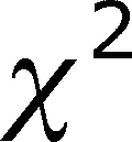
- The way to test for goodness-of-fit is to use a
Chi-square (
 ) test.
- The test is based on measuring the deviation
of the data from the expected outcome.
- First, you must calculate the expected outcome,
which is dependent on the circumstances of the test.
- Then you subtract the expected outcomes from
the observed outcomes.
- If you were to sum these deviations, they
would sum to 0 (this is an outcome of the fact that both the observed
and expected columns must sum to n, the number of observations).
- To avoid this, we have to get rid of the
- sign somehow.
- We could take the absolute value, which
we will not use, or we could square all of the deviations, so that negative
values become positive.
- Square all deviations.
- There is another problem. The size of the
sum of deviations will depend on the size of n. We partially correct
this by standardizing the deviation.
- Divide each deviation by the expected value
used to calculate that deviation.
- Sum all standardized deviations
- This sum is the
 value.
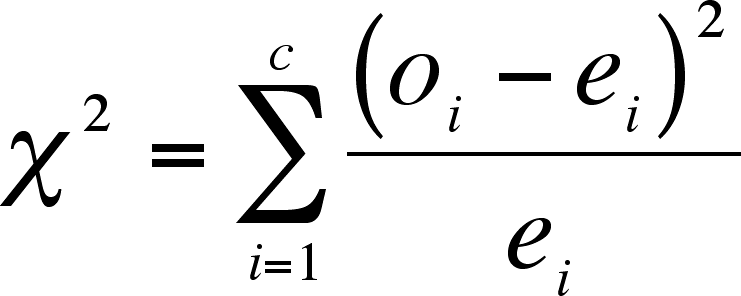
- Where o = number of observations in a category,
e = expected number of observations in a category, i is the index, and
c is the number of categories.
Evaluation of the  value
value
- First, select an
 -value. This is a necessary step for any statistical
test.
- The
 -values are not normally distributed.
- The
 distribution begins at 0 (the outcome when all observed
are the same as expected values).
- The right side is skewed so that the right
tail extends to infinity.
- The exact shape depends on the number of
categories and the assumption that the deviations between the expected
and observed values are due to random error only.
- Think for a moment about how the
 -value is calculated and the distribution
will make some sense.
- As the
 -value increases, it means that the gap
between the observed and expected values is increasing.
- If the gap is due to random error only,
then really large values of
 must be uncommon (low probability).
- The tail to the right represents the probability
of getting a
 -value equal to or larger than the calculated
  -value.
- Thus, the tail probability is a measure
of how unlikely a
 -value as large as the calculated value
is, a measure of how likely your
  -value is given that it due to random
error alone.
- If this probability is too low, then
you are forced to reject the idea that it is due to random error alone
and accept that something else is contributing to the gap between observed
and expected values.
- You are forced to conclude that your
expected values are not the correct values and your model is incorrect.
- The null and alternative hypotheses are:
- H0 : The
 -value is due to random error and the expected
values are an accurate prediction of the observed values
- HA : The
 -value is too large to be due to random error alone
and the expected values are not an accurate prediction of the observed values
- The
question you must answer is "How unlikely
is my
 -value?" This
means you must look up the probability of getting a
  -value as large or larger than the value for
your data in the table in the back of the book.
- d. f. = the number of categories - 1
- NOTE THAT THIS IS NOT THE NUMBER OF OBSERVATIONS
- 1
Nondirectional vs. Directional
- Goodness-of-fit null hypotheses are called COMPOUND NULL HYPOTHESES because each of the expected values (except the
last, which is fixed by the values of the others since the total number
of observations is fixed) is an independent hypothesis.
- This fact means that the test must be non-directional,
as the deviation for each of the independent nulls can be either + or
-, so no overall direction is necessarily true for the entire test. We
just know the observed didn't fit the expected very well.
- The exception to this is when the outcome
categories are just two (a dichotomous variable). Here, since only one
of the expected values is not fixed, then directionality is possible.
For an example, see the 2 x 2 contingency table below.
- Reject
the null if your
 is larger than the Table 9 entry for the
appropriate d. f. and the non-directional
  value divided in half.
Last updated November 12, 2012


![]() =
3/10 = 0.30
=
3/10 = 0.30
![]() (or
(or ![]() ),
given that the true proportion is p? Once
again, a metaexperiment is where to begin.
),
given that the true proportion is p? Once
again, a metaexperiment is where to begin.![]()
![]() value
valueis larger than the Table 9 entry for the appropriate d. f. and the non-directional
value divided in half.