|
|
|
|
|
|
|
|
|
|
|
|
|
|
Introduction: In this lab, we will go to a forest and not measure many of the things one might measure there. We will not, for instance, measure the density of trees or their average size, or the diversity of species. Hopefully, we will get some idea of this from simply walking through the forest and being observant. These are all important things to know, but they may not tell one much about the interaction among trees, which is what I would like us to concentrate on today. We will look for patterns in space. For sessile organisms, like plants or corals, the environment in which they develop and reproduce can not be changed by the organisms once they germinate (or settle out of the water column). Their environment is the immediate neighborhood. The neighboring trees are potential competitors, whether or not they are of the same species. When we observe such organisms, it may be possible to detect some interactions from their spatial pattern. Before we can do this, we should consider what patterns might be there and what they might mean.
If trees do not interact, the location of any tree would be independent of the location of any other (assuming that they fall to the ground independently too). This would lead to a random spacing of trees. A second possible pattern might be that trees are spaced evenly (like corn plants in a field). This pattern can be called either uniform, regular or "under-dispersed." Ask me during the lab how that last name came about. One thing that could give rise to regular spacing might be some kind of competition, such that there is a minimum distance between plants, as each plant commands the resources (light, moisture, nutrients) within its sphere of influence and this keeps other plants from growing there. A third possible pattern might arise when plants find the underlying substrate uneven in quality. If this is so, many plants may cluster within the patches of good quality, giving rise to short interplant distances within the patch, while distances between plants in different patches would be large, separated by the poor patches in between them. This would lead to two kinds of distances, very large and very small (with few intermediate distances). This pattern is called aggregated, contagious, clumped or "over-dispersed". There are many possible reasons for aggregated distributions other than patchy resources. Remember that I assumed a random seed fall when describing how random dispersion patterns arise. However, if a plant depends on an animal to disperse its seeds, then the behavior of the animal when doing so might lead to aggregated distributions. Other factors such as storms, disease, and insect infestation might also lead to clumping. Here is a challenge. Can you suggest another reason for a regular dispersion pattern other than interplant competition (other than human intervention)?
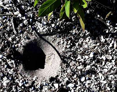
While pattern analysis is not a definitive proof of interaction (one would have to do an experiment to determine the real cause of the patterns), it is useful as a means of generating testable hypotheses about the interactions between trees. We will take an experimental look at the interaction among plants in another lab. In addition, we must remember that spatial pattern is important to all populations, without regards to the organisms that comprise the population. The antlion pictured above digs a pit and lies in wait at the bottom to eat whatever smaller insect falls into the pit and can't climb out. The pattern of other antlion pits in the neighborhood has a strong impact on the number of prey the antlion will get.
Gathering the Data:
Sampling Design:
When confronted with an object of study as large as a forest, or even a single species within the forest, it is rare that one can census the entire population. Therefore, what one must do is sample a subset of the entire population and draw conclusions about the whole from the sample. There are many ways to do this, and we will look at two today, quadrat sampling and transect sampling. Quadrat sampling subdivides the area into smaller blocks (= quadrats) and samples some of them. Transect sampling (of which there are many versions such as linear intercept, point-quarter, and the one we will use today, nearest-neighbor) samples only those individuals that occur at pre-determined points along a line(s) (= transect(s)) drawn through the sampling area.
A second consideration is whether or not one should stratify the sampling area. Unstratified sampling treats the entire area as unchanging or all individuals as equals. This might be true in cases where the there is little change in elevation or soil type within the area or in cases where individuals of all species and ages have similar resource requirements. Many times, one can easily see that there is a change in elevation or one may have a map of soil types within the area. There may be a physical feature which can obviously affect one side of the area of interest more than another (such as a river along one side). Mature individuals may use different resources than immatures or species may have different resource requirements. When this occurs, one can choose to stratify the sample, which means to subdivide the sampling so that some samples are taken from each of the different strata (low and high elevations, chalky and loamy soils, wet and dry soils, large and small individuals, different species). We will stratify our sampling into just two categories of trees: canopy trees and understory trees.
Quadrat Sampling of a Forest:
One must make four decisions about quadrats.
How large should they be?
This is a practical decision. The quadrat must be large enough so that more than one individual can reasonably fit into it and not so large that one can not count enough quadrats to adequately sample the population or forest. We will make our quadrats 12 m by 20 m.
How many are to be sampled?
Once again, this is a practical decision. There are eight groups in the class, and each will sample two quadrats for a total of 16 for the class.
How are we to count the individuals within a quadrat?
This decision is not simply a practical one. One may wish to consider all of the trees sampled as equivalent, so that one simple counts the number of stems of each species of interest. Often, the size of the individual is important. For trees, size can be considered from two perspectives. The amount of sunlight available for a forest plant is related to its height. Plants in the forest canopy receive direct sunlight, those below are shaded by the canopy plants. The amount of nutrients and water available to a plant is related to its cover area, the area of its crown of leaves (which is usually assumed to be circular). For small, understory trees and shrubs, this is measurable directly. For canopy trees, the basal area of the trunk (cross-sectional area at a pre-determined height from the ground) is substituted as it is usually directly related to the crown size above. However, for our purposes, we will stratify our sampling into canopy and understory trees and simply count the number of stems of each species in each category. You will have to decide if the tree is in the canopy or not.
Some practical considerations. If any part of a plants stem is in the quadrat, it is counted. We will ignore all plants that are less than 1 inch in diameter at breast height (often abbreviated dbh).
How are the quadrats to be placed within the sampling area?
There are many ways to do this, and we haven't the space to describe them all or even a reasonable subset. However, two things should be mentioned. Often one maps the entire area, divides it into square coordinates (like latitude and longitude on large maps) and randomly picks the coordinates at which the quadrats are placed. A second way is to use a transect to locate the coordinates by randomly choosing points along the transect to place the quadrats. We will use this method, since our study area (called Tornado Ridge) has a natural transect, the trail along the top of the ridge. We will locate our quadrats along the ridge at (pseudo)randomly chosen points.
Your data should take the form of a table, with category of trees found along one side as the rows and quadrat number along the top as columns.
Nearest-Neighbor Sampling:
This technique is based on one or more transects of the sampling area. The procedure is to walk along the transect and stop at random points. The minimum spacing should guarantee that no tree is sampled at two consecutive points. At each point, determine the nearest tree. Then find the nearest neighbor to that tree. Record the distance between nearest-neighbors. Measure the basal area of both neighbors. We will measure the basal area of canopy trees by wrapping a measuring tape around it at breast height to get the circumference. Later, you can convert this to basal area with the formula below
Do this for an understory (remember that the nearest neighbor must be another tree from the same category so the other member of the pair must be another understory tree) and a canopy tree (with the other member of the pair another canopy tree) each time you stop along the transect. Do this for 5 transect points (i. e., for 5 stops). Ignore any understory trees less than 1 inch dbh.
Data Analysis:
One of the ways in which organisms may interact is competition.
Quadrat data:
The three patterns (regular, random, and aggregated) can be easily detected with a statistic called the variance-to-mean ratio. We can symbolize this as s/m (by using the Greek symbols for variance and mean). First, you should organize you data into a frequency distribution of individuals per quadrat. Some quadrats will have contained 0 or 1 or 2 or 3 or more trees. For example, suppose that 4 quadrats had 2 trees, 6 quadrats had 3 trees, 5 had 4 trees, 2 had 5 trees, 4 had 6 trees and one had 8 trees. Then the we can then group the data as:
|
xi |
|
|
|
|
|
|
|
|
|
|
frequency |
|
|
|
|
|
|
|
|
|
Note that xi refers to the number of trees in a quadrat and frequency is the number of quadrats that contain xi individuals.
You can easily calculate the mean from such a table. First, add up all of the frequencies. This is the total number of quadrats. Then multiply each xi times its frequency and sum all products. This is the total number of trees in all quadrats. Now divide the total number of trees by the total number of quadrats and you have the mean trees per quadrat. This is half of the statistic.
Number of quadrats = sum of frequencies = 4+ 6 + 5 + 2 + 4 + 1 = 22
Number of trees = sum of (freq. x xi ) = (4·2)+(6·3)+(5·4)+(2·5)+(4·6)+(1·8) = 88
Mean = 88 / 22 = 4.0
|
|
|
|
|
|
(xi -m)2x Frequency
|
|
|
|
|
|
|
|
|
|
|
|
|
|
|
|
|
|
|
|
|
|
|
|
|
|
|
|
|
|
|
|
|
|
|
|
|
|
|
|
|
|
|
|
|
|
|
|
|
|
Variance = 56 / 21 = 2.67
s/m = 2.67 / 4 = 0.67
Now, why do we calculate such a statistic? It can be shown (we haven't the space here) that the three types of patterns all have different variance-to-mean ratios. So, the statistic can be used to infer the underlying spatial pattern. If the pattern is random, then the variance is equal to the mean and s/m is 1. If it is aggregated then s/m is more than 1. Remember that we get more small and more large vales than expected when the trees are clumped, and it is the large values that make the variance larger than the mean because you square the differences when calculating the variance and large differences result in big square terms. Finally, uniform or regular patterns have a variance-to-mean ratio less than 1.
So, we can see that our statistic is telling us that this population is underdispersed or regularly spaced in our example. The trees might be competing. However, there is one little problem. If the population were actually randomly spaced and we took a sample, we could not expect that the sample data would give us a ratio of exactly 1. It would be like flipping a coin ten times and betting your life that you get exactly five heads. Although we expect to get 5 heads, it is still a bad bet. Random chance can cause deviations from expectation. In our example here, the question is, "Is 0.67 an indication of regularity or is the real value 1 and we measured 0.67 due to some experimental error?". Put another way (as a statistician might ask it), "Is 0.67 significantly lower than 1? Well, there is a way to infer whether it is or isn't!
So, what would we expect if the distribution in our sample came from a randomly spaced population? We don't want to change the mean. We just want to know if our data is within reason of the mean or is it spread too far from the mean to accept that the spread is due to random error. There is a mathematical way to calculate the expected spread due to random error (with our mean). This distribution is called the Poisson Distribution and is worth learning as it predicts random outcomes from any data that can be summarized with a frequency table. According to the Poisson, the proportion (= percentage) of the quadrats one should expect in any class (= xi) can be calculated from the following simple formula.

This equation may be rather daunting, but I will walk you through it. The only new symbol is e, which is the base for natural or Naperian logarithms and is about 2.718 or so. Suppose you are trying to calculate how many quadrats you expect to get with 5 trees in them in our example (22 quadrats, mean of 4 trees per quadrat). First, you raise 4 (= m) to the 5th power (5 = xi) and divide this by 5 factorial (= 5 times 4 times 3 times 2 times 1 = 120). Then you take this quotient times e (= approx. 2.718) raised to the 4th power. Simple, right?
Proportion of quadrats with 5
trees =  =
= ![]() =
0.156
=
0.156
Or about 16% of the quadrats should have 5 trees. This is about 3.45 quadrats (remember that fractions are ok when you calculate them, although 0.45 quadrats doesn't really exist). Here are the complete set of expectations for our data. Notice that the sum of all the expectations equals 22. We can't expect any more or less than the total number of quadrats we actually sample. The problem is that the distribution goes to infinity, although we never got a quadrat with more than 8 trees. So, I lumped all of the classes above 8 in with 8 (notice the 8+) and this makes this class easy to calculate. Simply add the preceding classes together and subtract the sum from 1. Notice that for some of the classes (=xi's) that we expected to get something, even though we didn't actual see any quadrats with that number of trees (as in 0, ,1 or 7 trees/quadrat). You can't ignore a class simply because you didn't happen to get any data there! Also recall that 1! and 0! are equal to 1.
|
xi |
|
mxi |
xi! |
expected proportion |
expected number |
observed |
|
0 |
0.018 |
1 |
1 |
0.018 |
0.4 |
0 |
|
1 |
0.018 |
4 |
1 |
0.073 |
1.6 |
0 |
|
2 |
0.018 |
16 |
2 |
0.147 |
3.2 |
4 |
|
3 |
0.018 |
64 |
6 |
0.195 |
4.3 |
6 |
|
4 |
0.018 |
256 |
24 |
0.195 |
4.3 |
5 |
|
5 |
0.018 |
1024 |
120 |
0.156 |
3.4 |
2 |
|
6 |
0.018 |
4096 |
720 |
0.104 |
2.3 |
4 |
|
7 |
0.018 |
16384 |
5040 |
0.060 |
1.3 |
0 |
|
8+ |
|
|
|
0.030 |
1.1 |
1 |
|
|
|
|
Totals |
1.000 |
22 |
22 |
Ask yourself this. Am I sure that I know why both the expected number and observed columns sum to 22 and why the expected proportions sum to 1. If you do not, you are confused about this table and should ask your instructor for clarification. Notice that I had to calculate the expected proportions and numbers for 0, 1, and 7 trees per quadrat, even though I did not observe any quadrats with those trees. This can be a nuisance when you get one or two very large observations. This is when it is best to do the calculations with a computer spreadsheet program. If you need instruction about using such a program, tell me. I will set up some times for tutoring. A second point. Notice that the last category is 8+, not just 8. The Poisson distribution is infinite, and assigns probabilities to all values of xi greater than 8! We get around this by summing all of the proportions from 0 to 7 and subtracting this sum from 1. This difference is the value you should use for the last entry in the table, and it is the proportion of outcomes that should have 8 or more trees per quadrat.
As you can see, there is some discrepancy between the observed number and the expected number if the trees were spaced randomly. But, to get back to the central question, is this a significant difference between random expectation and our data? If not, then the distribution of the trees in our example are random. If the difference is significant, then they are regularly spaced. So, how do we decide on significance? This is subjective, so I as lab instructor will make a decision. A difference is significant if there is less than a 5% chance that the statistic calculated from the actual data could have resulted from a random pattern. So, now to the determination of just how likely the example's statistic (s/m = 0.67) is if we assume the actual pattern is random.
We will use a statistical technique called the Chi-square test (c2) to figure our chances. Its calculation is easy. For each xi, we have an observed and an expected value. Subtract the expected from the observed, square the difference and divide the difference by the expected value. The squared difference is a measure of how unexpected the data are (given the assumption of randomness) and dividing this by the expected value corrects for the fact that some data comes in ones, some in tens, some in hundreds, etc. Without this correction, we could not use the same test on data that comes in large values (like bacterial numbers) and data with small values (like tree quadrat data). The Chi-square value is the sum (for all xi)of these quotients.
|
xi |
observed |
expected |
obs-exp |
(obs-exp)2 |
(obs-exp)2/exp |
|
0 |
0 |
0.4 |
-0.4 |
0.16 |
0.4 |
|
1 |
0 |
1.6 |
-1.6 |
2.60 |
1.6 |
|
2 |
4 |
3.2 |
0.8 |
0.60 |
0.2 |
|
3 |
6 |
4.3 |
1.7 |
2.90 |
0.7 |
|
4 |
5 |
4.3 |
0.7 |
0.49 |
0.1 |
|
5 |
2 |
3.4 |
-1.4 |
2.07 |
0.6 |
|
6 |
4 |
2.3 |
1.7 |
2.92 |
1.3 |
|
7 |
0 |
1.3 |
-1.3 |
1.72 |
1.3 |
|
8 |
1 |
1.1 |
-0.1 |
0.02 |
0.0 |
|
Totals |
|
|
|
|
6.2 |
In order to evaluate this result, you have to use the attached table. You can read the probability of your results being random from this table. First calculate the degrees of freedom, which is the number of xi - 1 (9 - 1 = 8 in our example, remember that the 0 class adds one, so we start with 9, not 8). Your results are significantly different from random if your Chi-square value exceeds the one in the table. Since the value in the table is 15.5 and the value in the example is 6.2, we can conclude that we do not, in fact, have evidence that the spatial distribution of trees in our example is regular. Although 0.67 seems very much smaller than 1, a randomly distributed forest would give such a low value (through random error when taking the sample) more than 5% of the time.
Present the class frequency table; calculate the mean, variance, and variance-mean ratio; calculate the Poisson expectations for the data, and, finally, calculate the Chi-square value and tell what your conclusions are for the data the class has gathered on the spatial distribution of trees.
As a matter of disclosure, I must tell you that the conclusion you have reached is based on the size of the quadrats. A different quadrat size might lead to a different conclusion.
A last note about the statistics calculated here. Many statistical tests work better with large amounts of data than with small amounts. Both the Poisson and Chi-square calculations are subject to some error when the data in any category is too small. The rule of thumb for both is if any calculated expectation (expected number of quadrats) is less than 5, one normally combines xi's so that all expected values exceed 5. We might have done this here by grouping the xi's. However, we may have so little data here that this would not be particularly useful, so we will simply ignore this for this lab.
Nearest-Neighbor data:
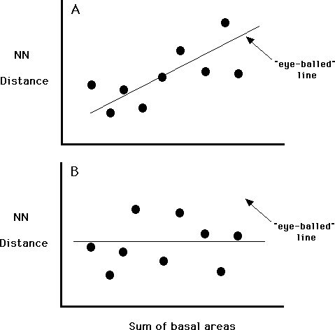
We will try to keep this analysis a bit shorter, although we will do this through simplification and not because there is any less real math behind a rigorous analysis of this kind of data. Let's just look for some evidence of competition. If we think of plant competition being based on gathering all of the resource within an "area of influence" then larger plants will have a larger area of influence than do smaller plants. A second assumption is that the areas of influence of competing plants can not overlap because one plant will remove the resource and leave the other plant at a disadvantage. Non-competing plants might have overlapping areas of influence, as neither can exclude the other. A final assumption is that the size of the basal area of a plant is related to that plant's area of influence. With these assumptions, we can look for competition. Simply graph the distance between nearest neighbors (y-axis) versus the sum of the basal areas of the two nearest neighbors. If our assumptions are correct and if the trees are competing, then we should be able to see an increase in NN distance with an increase in pair size. This relationship can be described with the line that best represents the points on the graph (as in Figure A). No relationship between the two things would lead to Figure B (which I made by moving only three of the points in Figure A). There are ways to draw this line mathematically, but we won't use them. We will simply "eye-ball" the best line. Construct a graph for canopy trees and a graph for understory trees from the class data and draw your conclusions about competition based on the graphs.
Thinking about the laboratory:
Below is a table for use in evaluating the statistics used in this lab.
|
Chi-square values (not in bold) |
| ||
|
|
| ||
|
|
|
|
|
|
|
| ||
|
|
|
|
|
|
|
|
|
|
|
|
|
|
|
|
|
|
|
|
|
|
|
|
|
|
|
|
|
|
|
|
|
|
|
|
|
|
|
|
|
|
|
|
|
|
|
|
|
|
|
|
|
|
|
|
|
|
|
|
|
|
|
|
|
|
|
|
|
|
|
|
|
|
|
|
|
|
|
|
|
|
|
|
|
|
|
|
|
|
|
|
|
|
|
|
|
|
|
|
|
|
|
|
|
|
|
|
|
|
|
|
|
|
|
|
|
|
|
|
|
|
|
|
|
|
|
|
|
|
|
|
|
|
|
|
|
|
|
|
|
|
|
|
|
|
|
|
|
|
|
|
|
|
|
|
|
|
|
|
|
|
|
|
|
|
|
|
|
|
|
|
|
|
|
|
|
|
|
|
|
|
|
|
|