|
BIOL 4120 Principles of Ecology
Phil Ganter 330 Harned Hall 963-5782 |
| |
BIOL 4120 Principles of Ecology
Phil Ganter 330 Harned Hall 963-5782 |
Modeling Density-Dependent Population Growth
Back to:
Lecture 11 Population Regulation
This is the first modification of the equation for exponential growth:
dN/dt = rN
A modification of this equation is necessary because exponential growth can not predict population growth for long periods of time. No matter how slowly a population grows, exponential growth will eventually predict an infinitely large population, an impossible situation. So we need to modify this growth rate to accommodate the fact that populations can't grow forever.
There are many ways to model the relationship between population size and b or d. The simplest is a linear relationship, such that a linear equation can be used to predict b (or d) given N:
d = d0 + zN
Take a moment to consider units, which are the key to understanding mathematical models. If d is an instantaneous rate of population change its units are individuals/(individuals*time). The numerator is obvious as we are changing the number of individual when a population grows or shrinks. The denominator means that the rate depends on time (as rates tend to do) and the individual. So r, b and d are all per capita rates. As z converts between N and d, its units must be 1/(individuals*time), so that when you multiply it by N individuals, you get the right units for d (be aware that one cannot add two numbers if they do not have the same units, a fact that is often assumed by writers of equations but forgotten by those reading equations).
We have to slightly change the equation for b, as the birth rate should decrease with mortality (given more individuals and the same resource base).
b = b0 - vN
Now rewrite the equation for exponential growth keeping in mind that r = b - d:
dN/dt = rN = (b - d)N
dN/dt = [(b0 - vN) - (d0 + zN)]N
or
dN/dt = [(b0 - d0) - (v + z)N]N
dN/dt = [(b0 - d0)/(b0 - d0)][(b0 - d0) - (v + z)N]N
dN/dt = (b0 - d0)[(b0 - d0)/(b0 - d0) - (v + z)N/(b0 - d0)]N
dN/dt = (b0 - d0)[1 - [(v + z)/(b0 - d0)]N]N
dN/dt = rN{1 - [(v + z)/(b0 - d0)]N}
We are almost there now. I hope you can see that it was useful to perform the not-so-obvious step as it gave us back an equation that is similar to one with which we are already familiar. Notice, however, that we have added a term to the original equation for exponential growth. It is this term that is the modification we are seeking: the term that alters population growth rates as the density of the population changes. This effect is called density-dependence in the sense that b and d are linearly dependent on the density of the population. Lets consider that term (I will call it the DD term) more closely as there are too many variables in it for convenience:
[(v + z)/(b0 - d0)]N
dN/dt = rN{1 - [1/K]N}
or
 .
.
This is the form I will use in class.
This form of the equation is called the Logistic Equation. When N is small, the DD term is near 1 as the N/K term is small, and the population grows at near maximal rate. Notice what happens as N increases. As N approaches K, the N/K term comes near to 1 and when subtracted from 1 the DD term gets smaller and smaller, indicating that the population is growing at only a fraction of its potential. Eventually K and N are equal and the DD term becomes 1 &endash; 1 or zero. Growth stops (the growth rate is 0) when N = K (look above at the definition of K). The population is stationary (neither growing nor declining) and we call this population size the carrying capacity. This term implies that this is the maximal number of individuals that can be sustained in that environment. K is in units of individuals but is related to the amount of resource present and the amount of resource needed per individual.
A word about the assumption of linearity. It is the simplest way to model the relationship between b, d, and N but it may not be very realistic. A curve of some sort is more likely to be realistic, as the effect of adding individuals may not be felt until some critical threshold in resource per individual has been crossed. Indeed, there may be an increase in birth rates (or a decrease in death rates) when individuals are added at low density (this is called the Allee effect after an ecologist interested in the benefits of living in groups). Below is a figure that shows the relationship between b, d, and K. Many other models have been used in which b declines with N and d increases, but the relationsip is a curve instead of the lines below.
In the diagram above, b0 and d0 are the Y-intercepts of the b and d lines respectively and v and z are the slopes of the lines. It it possible to calculate r, but only as b0 - d0 (the intercept values), the birth and death rates unaffected by density, as r is defined without any density effects. If you subtract the values at some density other than 0, you get the population growth rate at that density. K is easy to find because it is the point at which population growth is zero, and that will happen when b0 = d0, which is the intersection of the two lines.
The assumptions of the logistic include all of the assumptions found in the model it is based on: the exponential growth model with the exception that there be a constant b and d. To review those assumptions go to Modeling Exponential Growth. We modified the equation by violating the assumption of constant birth and death rates. In doing so, however, we have added other assumptions"
It is possible to use the rules of calculus to integrate the growth rate equation to calculate the population size at a given time if the initial population size (N0 is known). We won't do the math here, but will give the equation:
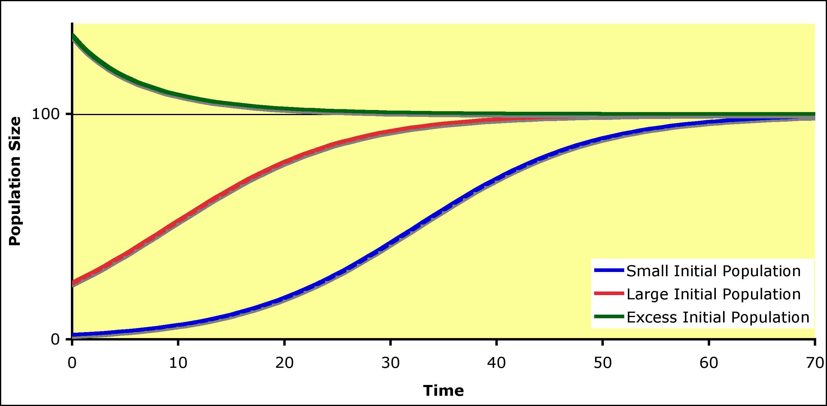
When you calculate growth rates with this equation and start with N near 0, you can plot a curve called a sigmoid curve (x-axis is time, y-axis is population size), which grows quickly at first, but the rate of increase drops off until it hits zero, at which there is no more increase in N. Due to the continuous nature of this equation, K is actually an asymptote, a limiting value that the equation never actually reaches. This is where one is reminded that the logistic is a model and will not behave exactly as a real population would, as a real population can grow by no less than one individual and this equation predicts growth (when close to K) of fractional individuals.
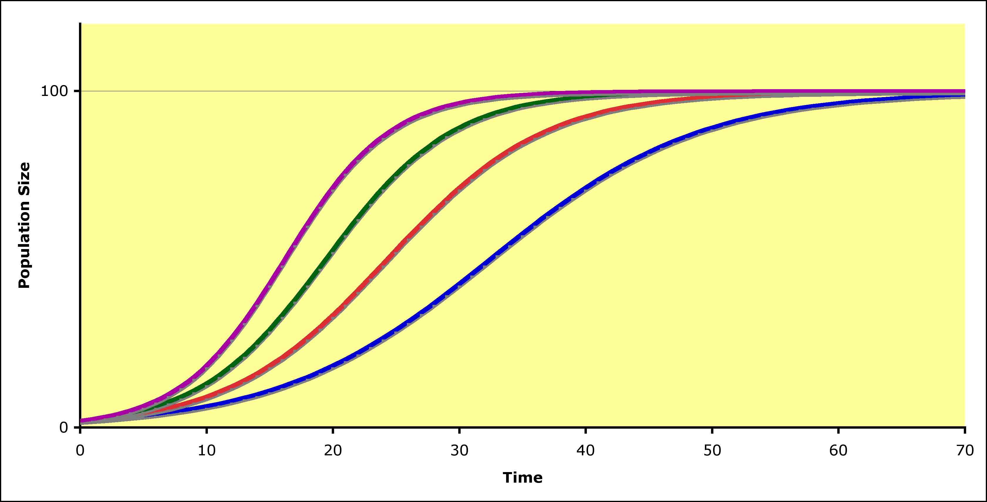
Let's look at the effect of changing some of the parameters in the prediction of future population size. We will begin with the prediction for a population with a K of 100, an r of 0.16, and a minimum initial population size of 2. The change in the population looks like this (blue line - Small Initial Population in the Key) - Remember K = 100:
Problems:
Literature Cited
Lotka, A. J. 1925. Elements of Physical Biology. Williams and Wilkins, pubs., Baltimore.
Verhulst, P. F. 1839. Notice sur la loi que la population suit dans son accroissement. Correspondence in Mathematics and Physics 10:113-121.
Last Updated on March 2, 2007