BIOL 4120 Principles of Ecology Phil Ganter 320 Harned Hall 963-5782
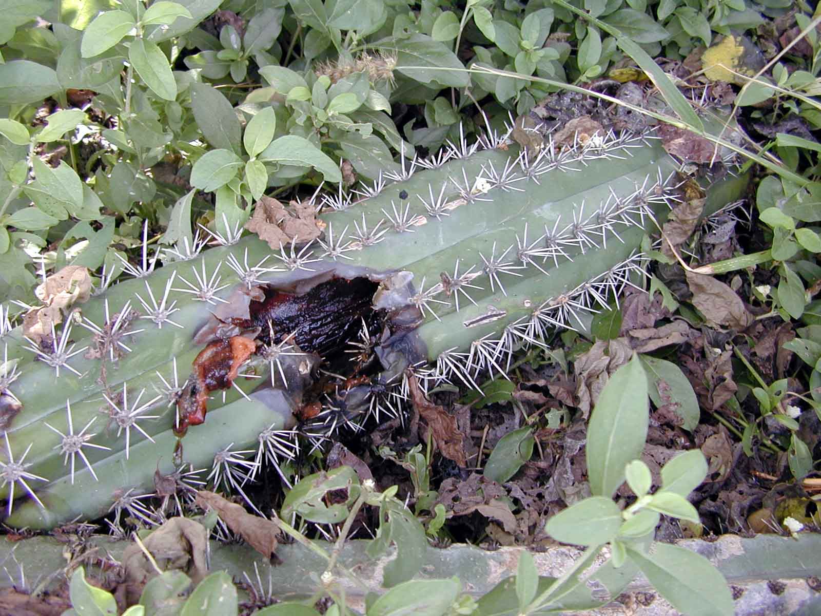
The damaged cactus arm above is home to a community of microbes and insects.  The populations of each species there are living in a temporary habitat and face the certainty of extinction when the damaged tissue has been consumed.

Lecture 10 Population Growth

Email me

Back to:

Overview - Link to Course Objectives

For more on the model of growth, go to Modeling Exponential Growth page

• Demography
• Life Expectancy
• Net Replacement Rate
• Generation Time
• Deterministic Models of Population Growth:
  • Geometric Population Growth
  • Exponential Population Growth
• Stochastic Processes and Models
• Population Extinction
• Terms

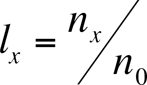
Describing a Population

Demography is the science of life tables

Life Tables are accounting of births and death in a population

Usually the life span of an individual is broken into stages (egg, larvae, etc.) or by age intervals or classes (0-5 years, 5-10, etc.)

Cohort - all of the individuals born at the same time

• x = the interval
• n_x = the number alive at the START OF THE INTERVAL
• l_x = age specific survivorship -- fraction of cohort alive at the START OF THE INTERVAL
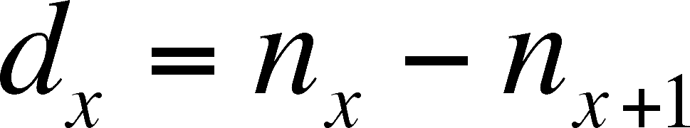
• d_x = age specific mortality -- number dying in the interval
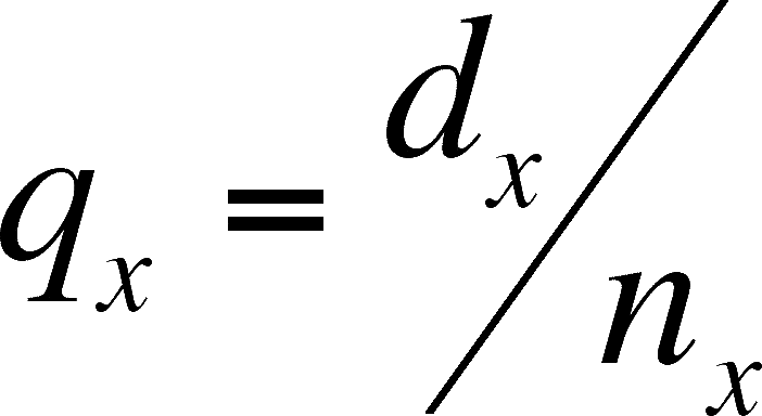
• q_x = age specific mortality rate -- death rate for individuals of a specific age
• e_x = age specific life expectancy - number of years left for an organism of a particular age.
  • Life expectancy is not always maximal at birth!!
• b_x = age specific natality -- number born in the interval
• m_x = age specific birth rate - the per female rate of offspring production for females of a particular age.
• R₀ = net replacement rate = the number of females alive in the next generation for each female alive in the present generation.
• T_c = generation time -- the average time between a birth of a member of the cohort and the birth of a member's offspring
• Age specific means that the parameter varies with the individual's age

By convention, the first age interval has the notation 0, so the number in the cohort at the start is n₀.

• n₀ is also the Cohort size - a Cohort is the group of newly born organisms that are followed throughout their lives in the life table

Another convention (especially for human life tables) is to multiply the number in the l_x column by 1000 (if it is actually 0.562, then it reads 562).

However, if you wish to calculate the net replacement rate (equation given below), then you must either convert l_x back to a proportion or you will be calculating the number of females in the next generation per 1000 females alive in the present generation!

If we plot log (nx) versus age, we can see where most of the mortality occurs by where the numbers drop

• Type I Mortality curve
  • most mortality comes late
  • characteristic of K-selected organisms (us)
  • often associated with organisms that put a lot of resources in to postnatal care
• Type II Mortality curve
  • mortality constant throughout life
  • results in a constant proportion of each age class surviving
  • birds are the classic example
• Type III Mortality curve
  • most mortality comes early
  • characteristic of r-selected organisms
    • many exceptions to this generality

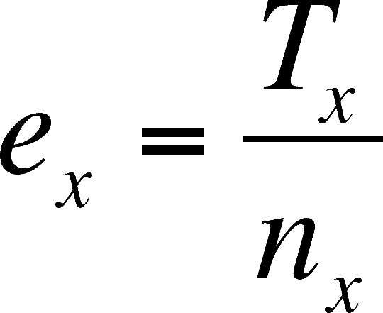
Life Expectancy

To calculate e_x, we will need to tack on another pair of columns to make it easier to do. This column is L_x, the average number alive in interval x. This is simple to do:

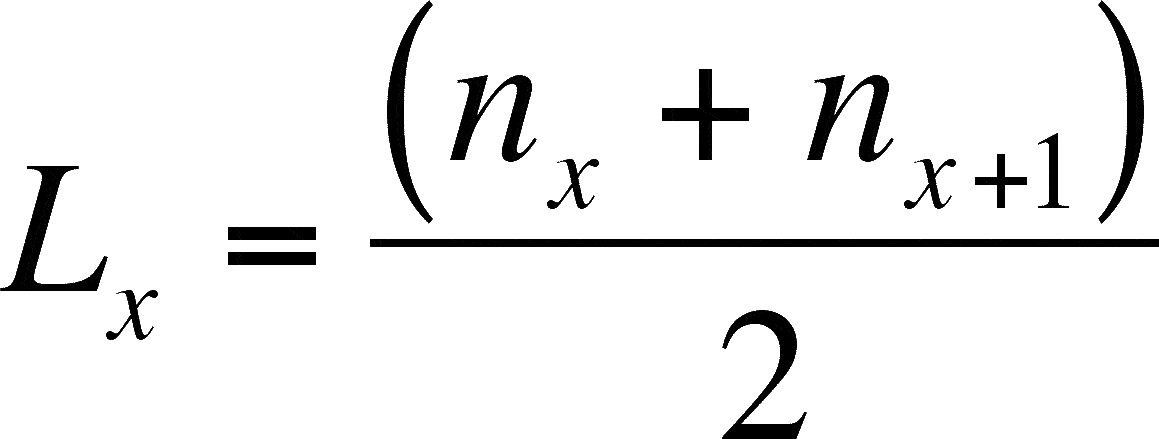
From this column, we can get Tx, which is the sum of all of the Lx values from x until the age that the last member of the cohort dies (this is symbolized by L°).

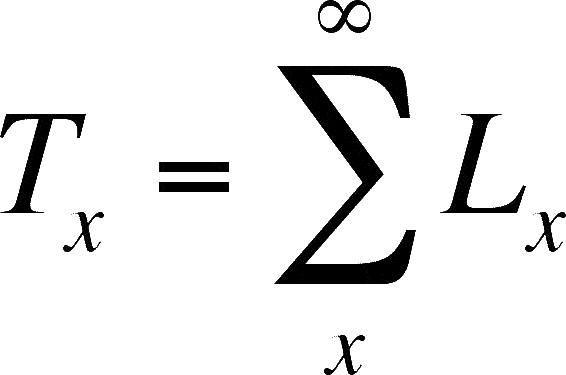
Life expectancy at age x is simply the average number of years lived by members of the cohort that are age x.

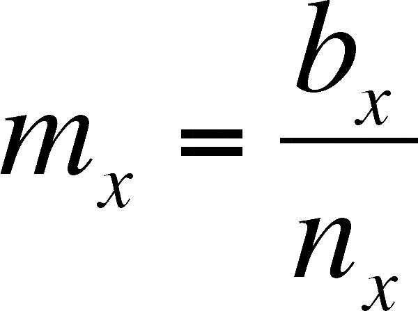
Net Replacement Rate

Net replacement rate is a measure of relative growth. It is the number of females alive in generation x+1 for each female alive in generation x. If it is greater than 1, the population is growing as there are always more females alive in the next generation than in the present. If less than 1, the population is decreasing (less than 1 female in the next generation per each alive in the present generation), and a net replacement rate of 1 means each female is exactly replaced in the next generation, so the population is stable, neither growing nor declining.

If we eliminate the males and add a column containing births, then we can calculate the net replacement rate. First, we must calculate the per capita birth rate (mx) for females of age x (females only!)

The net replacement rate is the sum of age-specific birth rates times the age specific survivorship. This means that an age class's contribution to the replacement rate must take account of the probability of surviving to that age.

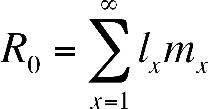
The net replacement rate is a measure of population growth rate.

If it is 1, then the population in neither growing or declining in size (a stable population).

If it is less than 1, the population is declining by that proportion each generation (if it is 0.5, then the population will be half as big each generation).

A value over 1 indicates a growing population (a value of 2 is a population that doubles each generation).

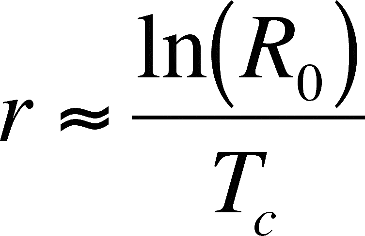
Generation Time

Assume that the net replacement rate is near 1. If so, we approximate the generation time as:

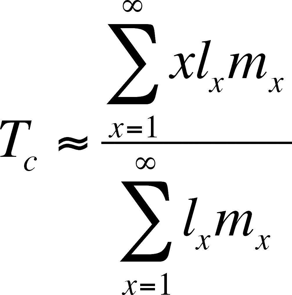
The approximation is due to the discrete nature of a life table, versus the continuous nature of time (an integral approach would get the exact figure)

Deterministic Models of Population Growth:

A model is a description of a natural phenomenon

Can be

• verbal (a story)
• pictorial (graphs)
• mathematical (equations)

Can be:

• Deterministic - exactly predicting the outcome
• Stochastic - giving a range of possible outcomes, with a probability of each occurring

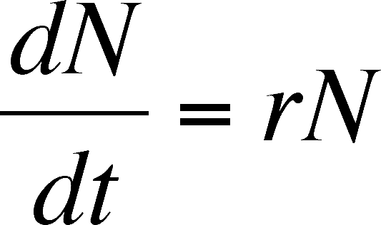
Geometric (discrete generations) and Exponential (overlapping generations) Population Growth

Geometric Population Growth

• Non-overlapping generations (univoltine insects, annual plants, etc.) use discrete equations
• The change in size over a generation is:
  • 
• And the change over many generations is:
  • 
• N_t the population number after t generations, N₀ is the original population size

   

  Exponential Population Growth

  Populations with overlapping generations (us!) use continuous equations

• Overlapping generations means that births are continuous, so that dividing young into cohorts is purely arbitrary
  • humans (and many great apes) have overlapping generations as do many small mammals (rodents) and many invertebrates in non-seasonal environments
  • Many mammals in seasonal environments do not have continuous generations, as all young are born within a few weeks of one another during a particular season
• Continuous equations describe events that occur continuously (like births in a population with overlapping generations)
  • Calculus is best to describe continuous events
  • Matrix algebra often better when generations are discrete
• Predicting the future size of a population based on its current size and assuming exponential growth can be done with the following equation:
• 
• r is the intrinsic rate of natural increase and is an instantaneous rate, which the book points out is the difference between the instantaneous birth and death rates (r = b - d), and is a per capita rate (an average rate taken over all individuals in the population)
• we can approximate this as (approx. because gen. time is approx.)



• the rate of increase in the population (dN/dt) is dependent on two factors:
  • the intrinsic rate of natural increase, which is one individual's contribution to population growth and so doesn't tell what the whole population is doing
  • the population size (larger populations increase by more individuals)

  

  The instantaneous rate of increase of a population (dN/dt) is the result

  For more on this topic, go to Modeling Exponential Growth page

Stochastic Processes and Models:

Stochastic demographic process are random changes in birth and death rates from year to year

• Random here means unpredictable
• Random fluctuations in demographic processes can arise from two sources
  • Environmental Stochasticity - fluctuations in edaphic or biotic factors that influence demographic processes, such as temperature and disease causing changes in the mortality rate.
  • Demographic Stochasticity - fluctuations in death or birth rates that are not caused by environmental sources.  These fluctuations may be due to genetic changes (perhaps due to Genetic Drift) or to random alterations of organisms physiology.

We can include stochastic change into our demographic models

• Deterministic models make specific, unique predictions about the size of populations at a specific time in the future - these are the models we have dealt with so far.
• Stochastic models are usually based on deterministic models, but make allowance for the fact the things vary in the real world

Predictions of population size made using stochastic models are couched as probability distributions of possible population sizes

• X axis is the size of the population at some time in the future
• Y axis is the probability of the population being at some particular size

  One would say that the size of a population is predicted to be 1232 organisms in six months if using the prediction from a deterministic model.

  One would say that, in six months, there is a 95% chance that the population will be somewhere in the range of 985 to 1456 if using the prediction from a stochastic model.

  In general, the longer in the future you try to predict population size, the larger the range of possible sizes

Population Extinction

Populations go extinct for many reasons

Some populations are, by nature, destined for extinction because their habitat is temporary

• many microbes live in situations that are temporary (my yeast are an example)
• plants that colonize openings in the forest live in habitats that will return to forest and become unsuitable for them
• populations of protists in temporary ponds

Some populations go extinct because of some unusual climatic event (very cold spell, flooding, severe storm, volcanic eruption [not really climatic]

Some populations go extinct due to Habitat Alteration by human activity

Probability of extinction is related to population size

smaller populations have a higher probability

Allee effect - the negative effects felt by populations that are smaller than some critical value (which is specific to each species)

• failure to find a mate
• Genetic drift may fix alleles in the population that are harmful (increase death rate or decrease birth rate)
• Inbreeding will increase the frequency of homozygotes (and, therefore, reduce heterozygosity) at loci with more than one allele present in the population
  • Homozygotes are sometimes less fit and may expose some recessive alleles, normally masked by the dominant gene in heterozygotes
  • Individuals with one or more detrimental alleles made homozygous by inbreeding may not be able to survive and reproduce in the population's environment.

Terms

Demography, Life Tables, Cohort, n_x, l_x, d_x, age specific mortality, q_x, age specific mortality rate, e_x, age specific life expectancy, b_x, age specific natality, m_x, age specific birth rate, R₀, T_c, generation time, Age specific, n₀, Type I Mortality curve, Type II Mortality curve, Type III Mortality curve, Life Expectancy, Net Replacement Rate, Generation Time, Model, Verbal Model, Pictorial Model, Mathematical Model, Deterministic Model, Stochastic Model, Geometric Population Growth, Non-overlapping generations, Discrete Equations, Exponential Population Growth, Overlapping generations, Continuous Equations, Intrinsic Rate of Natural Increase, Environmental Stochasticity, Demographic Stochasticity, Determinstic models, Stochastic models, Habitat Alteration, Allee effect, Genetic drift, Inbreeding

Last updated February 4, 2007