
|
BIOL 3110
Biostatistics
Phil
Ganter
301 Harned Hall
963-5782
|
Blackberry flower
|
|
Analysis of Categorical Data II
Chapter
10 (4th ed.)
or Chapter 10 (all but 10.1, 3rd ed.)
Email me
Back to:
Unit
Organization:
Problems:
Problems
for homework
- 3rd Edition -
10.13, 10.17, 10.21, 10.29, 10.31,
10.40, 10.48, 10.52, 10.55, 10.65,
10.68, 10.70, 10.74,
10.88
- 4th edition
- 10.2.1,10.2.4, 10.2.8, 10.3.4, 10.4.1,
10.5.2, 10.5.6, 10.6.2, 10.7.3, 10.8.3, 10.9.5
Suggested
Problems
- 3rd Edition - 40
(Fishers), 42 (Fishers)
- 4th edition
- 10.4.3
Go back
to the first lecture and brush up on data types.
- In
this lecture, we will cover analysis of categorical data.
- Categorical
data is data that is sorted into different qualitative
categories, not by a measured value.
- Sex,
color, genotype, are examples of categorical data. Each
observation fits into one category (male or female; red,
green or blue; AA, Aa, or aa).
2 x 2 Contingency Tables
Comparing
associations among factors
- Members
of a population can often be categorized based on more than one factor
(usually many factors). Every TSU student can be categorized by matriculation
status (matriculated full-time, matriculated not full-time, non-matriculated)
or by age or by residency or by sex or.... etc. One common type
of question we ask is:
- Is
there an association between (or among) factors? Note that
factor here means the same as variable.
- Are
males more likely to smoke than females?
- Does
level of unsaturated fat in the diet correspond to the risk of heart attack?
- To
answer these questions, we have to be more exact when we ask the question. We
are really asking if one factor is independent of the other
- Independence
here is the independence we have already discussed - that one factor does
not influence the other
- If
we couch the question in terms of probability, then we can develop methods
to answer the question based on what we know about probability
- Is
the probability that males smoke greater than the probability that females
smoke?
- Is
the probability that those who eat high-fat diets have heart attacks greater
than the probability that those who eat low-fat diets have heart attacks?
- CONTINGENCY
TABLES are
tables where one can contrast one factor/variable (the columns) versus
a second factor/variable (the rows).
- They are called contingency tables because we
are investigating if one variable's outcome is contingent (= dependent) on
the other variable.
- A 2 X 2 CONTINGENCY TABLE (said 2-by-2) is the simplest contingency
table where each variable has only two possible outcomes.
- Each of the combinations of of the variables get
a CELL of its own.
- To
test whether or not one variable is affecting the other, we need to have
an idea of what to expect if there is no association between the variables.
This means we need an expected that we can calculate.
- The
null hypothesis for a contingency table is that the proportion of
variable A in each category of A should be independent of which category
of variable B we are looking at.
- In terms of the example above,
the null hypothesis is:
H0: Pr{smoking|male}
= Pr{smoking|female}
- In English: the null hypothesis
is that the probability of smoking given that someone is a male is
equal to the probability of smoking given that someone is a female
- How
do we estimate these probabilities?
- We do this by using the MARGINAL TOTALS,
the totals at the margins of the table below:
| |
Variable
A |
|
Margin |
| Variable
B |
Category A1 |
Category A2 |
|
| |
| Category B1 |
21 |
4 |
25 |
| Category B2 |
8 |
32 |
40 |
| |
Total
# |
| Margin |
29 |
36 |
65 |
- The marginal totals for
Variable B (25 and 40) divided by the grand total (65) give
us our estimate of the frequency of categories B1 and B2
independent of Variable A.
- The marginal totals for
Variable A (29 and 36) divided by the grand total (65) give
us our estimate of the frequency of categories A1 and A2
independent of Variable B.
- So
we can use these marginal frequencies to get the expected proportion
of observations in each of the four
cells:
- (29/65) * (25/65) = 0.17
- (29/65) * (40/65) = 0.27
- (36/65) * (25/65) = 0.21
- (36/65) * (40/65) = 0.34
- These
are our expected probabilities (remember the connection between frequency
and probability) for all four outcomes GIVEN THAT VARIABLE A AND B ARE
INDEPENDENT!
- Why is this a given? Because we calculated
each probability as the product of two independent probabilities - this
is the null assumption
- To
do the test, we need to go beyond calculating the expected probability
of being in each cell. We need to calculate expected number of observations
in each cell, given the null assumption. This is easy to do because
we already have the expected probabilities
- The
expected outcome then are (simply multiply the proportions by the total,
65):
| Expected
Outcomes |
| |
Variable
A |
|
| Variable
B |
Category A1 |
Category A2 |
| Category B1 |
11.15 |
13.85 |
| Category B2 |
17.85 |
22.15 |
Total |
| |
65.00 |
- You now have a set of observations
and a set of expectations from which to calculate a
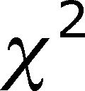 . In this case it is 25.5
- The chi-square distribution tell us the
probability of getting a value as large as we actually did
IF THE NULL HYPOTHESIS WERE TRUE
Evaluation
of the  value
value
- First, select an
 -value. This is a necessary step
for any statistical test.
- The degrees of freedom are the
number of rows -1 (r - 1) times the number of columns -1 (c - 1)
(r - 1) * (c - 1) = 1 * 1 = 1
- The
null and non-directional alternative hypotheses are:
H0 :
Variables A and B are independent
HA :
Variables A and B are dependent
H0: Pr{A|B1}
= Pr{A|B2}
HA: Pr{A|B1}
not equal to Pr{A|B2}
- Reject
the null if your
 is
larger than the Table 9 entry for the appropriate d. f. and the
  value.
- The directional alternative
hypotheses are:
HA1: Pr{A|B1}
> Pr{A|B2}
or
HA2: Pr{A|B1}
< Pr{A|B2}
- First
you have to check to see if the alternative of interest has actually occurred.
- If we choose HA1
above, then we would proceed because 21 of 28 A1 outcomes
were in B1 but only 4 out of 36 A2 outcomes were in B1
and this is as predicted by HA1
- If we choose HA2 above, then
we would not proceed because 21 of 28 A1 outcomes were in
B1 but only 4 out of 36 A2 outcomes were in B1 and this
is not as predicted by HA2
- Reject the null if your
 is larger than the Table 9
entry for the appropriate d. f. and the
  *2 value.
- Notice that we have look up
a value twice the alpha-value, which makes the cut off
 -value smaller and, so, a
smaller deviation will allow one to reject the null
hypothesis.
What have
we tested here?
- In
the non-directional case, we have asked if the two variables
are independent of one another or if they are associated.
- If we accept the null, we are
saying that Variable A and B are INDEPENDENT of one another.
- The outcome of A does not
depend on B and vice-versa.
- If
we accept the non-directional alternative hypothesis, we are saying that
variables A and B are ASSOCIATED.
- Association means that the
outcome of one corresponds to the outcome of the other.
- In our example, if you get A1,
then you also expect B1, but if you get A2, then you expect
B2.
- In
the directional case, we have asked if the association between two variables
goes in a particular direction
- If
we accept the directional alternative, we accept that the two variables have
a particular association (as defined by our choice of alternative hypothesis)
FISHER'S
EXACT TEST
This is a test that is an
alternative to the  for contingency tables.
- Exact because it gives the exact
probability of getting the cell values given the marginal totals.
H0: The
probability of infection is independent of the genotype
of the plant.
HA:
(directional) the probability of infection is lower for
aa than for other genotypes.
- Suppose that there are two
three genotypes but that the A allele is completely dominant.
You think the aa genotype might be useful if it shows
resistance masked by the dominant allele. So you set up an
experiment to test this. Plots of plants are exposed to the
fungal spores and the appearance of infected individuals is
noted. Plots are monocultures of plant genotypes. The
results:
| |
Genotype |
Frequency |
Margin |
|
| Infected |
AA or Aa |
aa |
|
|
Ways of getting
3 out of 16 |
| |
|
|
|
|
|
560 |
| Yes |
13 |
3 |
0.23 |
16 |
Ways of getting
10 out of 17 |
| No |
7 |
10 |
0.77 |
17 |
|
19448 |
| |
Total # |
Ways of getting
13 out of 33 |
| Margin |
20 |
13 |
|
33 |
|
573166440 |
| |
Probability |
0.019001 |
| |
| |
Genotype |
|
Margin |
|
|
| Infected |
AA or Aa |
aa |
|
|
Ways of getting
2 out of 16 |
| |
|
|
|
|
|
120 |
| Yes |
14 |
2 |
0.15 |
16 |
Ways of getting
11 out of 17 |
| No |
6 |
11 |
0.85 |
17 |
|
12376 |
| |
Total # |
Ways of getting
13 out of 33 |
| Margin |
20 |
13 |
|
33 |
|
573166440 |
| |
Probability |
0.002591 |
| |
|
| |
Genotype |
|
Margin |
|
|
| Infected |
AA or Aa |
aa |
|
|
Ways of getting
1 out of 16 |
| |
|
|
|
|
|
16 |
| Yes |
15 |
1 |
0.08 |
16 |
Ways of getting
12 out of 17 |
| No |
5 |
12 |
0.92 |
17 |
|
6188 |
| |
Total # |
Ways of getting
13 out of 33 |
| Margin |
20 |
13 |
|
33 |
|
573166440 |
| |
Probability |
0.000173 |
| |
|
| |
Genotype |
|
Margin |
|
|
| Infected |
AA or Aa |
aa |
|
|
Ways of getting
0 out of 16 |
| |
|
|
|
|
|
1 |
| Yes |
16 |
0 |
0.00 |
16 |
Ways of getting
13 out of 17 |
| No |
4 |
13 |
1.00 |
17 |
|
2380 |
| |
Total # |
Ways of getting
13 out of 33 |
| Margin |
20 |
13 |
|
33 |
|
573166440 |
| |
Probability |
0.000004 |
- Only the top part of the table
represents the outcome of the experiment (the data in black).
- The data in maroon
represents hypothetical situations discussed below.
- We need to know how likely is
this table, assuming that the marginal totals are fixed.
- Remember, that, since the
marginal totals are unchanging, if we know the
probability of the outcomes for one category of one
variable, we know the outcomes in the other cells, so we
need to find the probability of the outcome in a single
cell.
- The likelihood of the table
depends on the number of ways to construct the table with
the given cell entries divided by the total number of
ways to get the marginal totals
- These "number of
ways" are combinatorials, just like we worked with
when learning the binomial.
- The numerator is the
product of the number of ways of getting 3 successes out
of 16 trials (= 16!/((3!)*(13!)) = 560) times the number
of ways to get 10 successes out of 17 trials (=
17!/((10!)*(7!)) = 19,448), so the numerator is 560*19,448 = 10,890,880
- The denominator is the number
or ways to get 13 out of 33 trials = 33!/((20!)*(13!)) = 573,166,440
- The
probability is 10,890,880
/ 573,166,440 =
0.019
- But this ignores that there are
situations which give one more support for the rejecting the
null than the total experiment.
- These are the situations in
maroon above.
- Each one represents an
outcome that supports the directional HA , so
we have to add the probability of these outcomes to the
probability of the actual outcome.
- The
new numerator is the product of the number of ways of getting
2 successes out
of 16 trials (= 16!/((2!)*(14!)) = 120) times the number
of ways to get 11 successes out of 17 trials (=
17!/((11!)*(6!)) = 12,376), so the numerator is 120*12,376
= 1,485,120
- The denominator is the number or ways to
get 13 out of 33 trials = 33!/((20!)*(13!)) = 573,166,440
- The
probability is 1,485,120
/ 573,166,440 = 0.00259
- Once
this is done for all "worse cases", we
see that the probability of getting this outcome or one more in line
with HA is:
- Pr{this table) = 0.019 +
0.00259 + 0.000173 + 0.000004 = 0.0218
- If we have an alpha-value
of 0.05, then we reject the null and accept the
alternative.
- Notice that this is a directional
alternative. We will stop here and do the non-directional only if
we have time.
Confidence Intervals for Differences
between Probabilities in 2 x 2 tables
- If
you see the 2 x 2 table as two samples with two levels of a variable observed
in each, then you can ask if the probabilities differ between samples by
constructing a confidence interval for
the difference between the probability of some outcome within
each sample.
| |
Sample 1 |
Sample 2 |
| Category 1 |
x1 |
x2 |
| Category 2 |
n1 - x1 |
n2 - x2 |
| |
| Totals |
n1 |
n2 |
- If we define n1 and
n2 as the marginal totals of the columns (each
column is a different sample), we can define p1
and p2 as the probability of getting category 1 in
the two samples.
- We can ask if this
probability is the same in each sample.
- Define
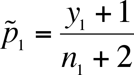 and
and
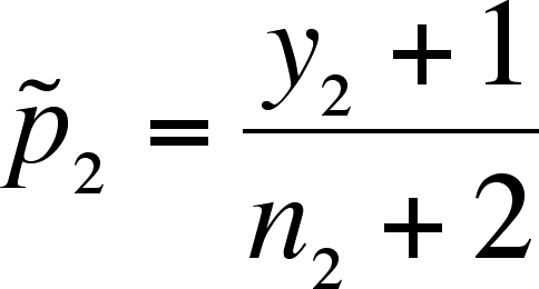 .
.
- Note that the addition
of 1 to the numerator and 2 to the denominator is a
correction for bias at small sample size.
- What
is needed is a standard error of the difference and a z value (which depends
on the
 -level
you want for the confidence interval - we will use the 95% confidence level
recommended by the book, which is 1.96)

- Then the confidence interval
is:

- If the CI includes 0, then it is possible (at that level of confidence)
that there is no difference between the samples. Concluding this
is the same as accepting the null hypothesis of no difference.
- Notice
that this is a way of doing a parametric test on categorical data.
r x k Contingency Tables
- There is no difference between this
procedure and the 2 x 2 we have already done.
- We just have more cells for
which we need to calculate expected numbers of outcomes and
we have to do the with more than 4 categories (r*c
categories, to be exact).
- An example will suffice:
- We will expand the previous
example to four rows by three columns.
- Notice that the expected
proportions still total to 1, and the observed and
expected totals are still equal to one another.
- Each expected proportion
cell is still the product of the row and column marginal
totals divided by the square of the total number of
outcomes.
| Actual Outcomes |
| |
Variable
A |
Margin |
| Variable
B |
Category A1 |
Category A2 |
Category A3 |
|
| Category B1 |
21 |
17 |
14 |
52 |
| Category B2 |
16 |
11 |
8 |
35 |
| Category B3 |
7 |
5 |
4 |
16 |
| Category B4 |
3 |
0 |
1 |
4 |
| |
Total # |
| Margin |
47 |
33 |
27 |
107 |
| |
| Expected
Proportions |
| |
Variable
A |
|
| Variable
B |
Category A1 |
Category A2 |
Category A3 |
| Category B1 |
0.21 |
0.15 |
0.12 |
| Category B2 |
0.14 |
0.10 |
0.08 |
| Category B3 |
0.07 |
0.05 |
0.04 |
| Category B4 |
0.02 |
0.01 |
0.01 |
Total |
| |
1.00 |
| Expected
Outcomes |
| |
Variable
A |
|
| Variable
B |
Category A1 |
Category A2 |
Category A3 |
| Category B1 |
22.84 |
16.04 |
13.12 |
| Category B2 |
15.37 |
10.79 |
8.83 |
| Category B3 |
7.03 |
4.93 |
4.04 |
| Category B4 |
1.76 |
1.23 |
1.01 |
Total |
| |
107.00 |
| Chi Square |
| |
0.1 |
0.1 |
0.1 |
|
| 0.0 |
0.0 |
0.1 |
| 0.0 |
0.0 |
0.0 |
| 0.9 |
1.2 |
0.0 |
Total |
| |
|
2.49 |
| Pr{Greater
chi-square) |
0.87 |
| df
= (r-1)*(c-1) = |
6 |
- As you can see, there is no
evidence that this table differs from the marginal expectations.
- The
 is only 2.49 and the
probability of such a large is 87%, far larger than the usual
0.5
  -level (the d. f. = (r-1)*(c-1) = (4 -
1)*(3 - 1) = 6.
- Notice that each Variable A
category declines from A1 to A3, no matter which Variable B
category you are looking at.
- The Variable A trends are INDEPENDENT
of Variable B and the difference between the observed and the
expected is due to random error.
- What if that were not true. What if
one of the Variable B categories bucked the trend?
- In the table below, Variable A
had the opposite trend in Category B3, increasing from A1 to
A3.
- By the way, the expected
proportions have been skipped as I have used the formula
(RowMarginal*ColumnMarginal)/Total to go straight to the
expected number of outcomes.
| Actual Outcomes |
| |
Variable
A |
Margin |
| Variable B |
Category A1 |
Category A2 |
Category A3 |
|
| Category B1 |
21 |
17 |
14 |
52 |
| Category B2 |
16 |
11 |
8 |
35 |
| Category B3 |
1 |
4 |
11 |
16 |
| Category B4 |
3 |
0 |
1 |
4 |
| |
Total # |
| Margin |
41 |
32 |
34 |
107 |
| |
| Expected
Proportions |
| |
Variable
A |
|
| Variable B |
Category A1 |
Category A2 |
Category A3 |
| Category B1 |
19.93 |
15.55 |
16.52 |
| Category B2 |
13.41 |
10.47 |
11.12 |
| Category B3 |
6.13 |
4.79 |
5.08 |
| Category B4 |
1.53 |
1.20 |
1.27 |
Total |
| |
107.00 |
| Chi
Square |
| |
0.1 |
0.1 |
0.4 |
|
| 0.5 |
0.0 |
0.9 |
| 4.3 |
0.1 |
6.9 |
| 1.4 |
1.2 |
0.1 |
Total |
| |
|
|
15.95 |
| Pr{Greater
chi-square) |
0.01 |
| df
= (r-1)*(c-1) = |
6 |
- Look at the difference this
change has made in the value of
 (once
again, the d. f. = (r-1)*(c-1) = (4 - 1)*(3 - 1) = 6. Now the Pr{greater
  -value} <0.01,
below the 0.05
  -level.
- This means that the trend
in Variable A DEPENDS on which category
of Variable B.
- Variables A and B are NOT
INDEPENDENT.
Paired Data and 2 x 2 Tables
- If your data is paired, it may be
possible to use categorical analysis to understand the
independence/dependence between outcomes for paired data. An
example will illustrate.
- A researcher wants to know
about the probability of attack of a newly developed bean
variety by a fungal pathogen. The data comes from plots of
the beans planted by farmers throughout Tennessee. Either the
plot is attacked by the fungus or it is not. Data is
collected for two years from the same plots and is presented
in the table below.
- The
pairing comes from the same plots being utilized each year so individual
plots can affect
two data points.
| |
Second
Year Infected? |
| yes |
no |
| First year Infected? |
yes |
67 |
165 |
| no |
210 |
31 |
| |
yes |
no |
| First year Infected? |
yes |
n11 |
n12 |
| no |
n21 |
n22 |
| |
|
| (n12
- n21)2 |
2025 |
| n12
+ n21 |
375 |
| chi-square |
5.4 |
| d. f. |
1 |
| Probability |
0.02 |
| alpha
-value |
0.05 |
| conclusion |
reject
null |
- n11 and n22
represent CONCORDANT pairs, those that did not have
an infection either year or had it both years.
- n12 and n21
represent DISCORDANT pairs, those that either
developed the infection in the first year and lost it the
second or developed it only in the second year.
- H0 for this analysis is
that the year did not make any difference in the probability of
the plot of beans being attacked by the fungus.
- H0 : a discordant
pair is just as likely to be yes- no as no-yes.
H0 : Pr{yes-no} =
Pr{no-yes} = 0.5
McNEMAR'S
TEST
- This test uses the
 test for the expected 0.5
distribution and is calculated as
 = (n12 - n21)2/(n12
+ n21), with 1 d. f.
- In the case above, it appears that
the years were not independent. It was more likely that plots
that were infected in only one year were more likely to be
infected in the second year than in the first.
Relative Risk and the Odds Ratio
- One often hears on the news some
reporter saying something like:
- "A
study just published in the Journal of the American Medical Association
reports that
listening to pop music increases a persons risk of dermatitis
three times."
- You almost never hear
scientists in areas other than clinical medicine report their
findings in this same way, but clinical researchers often do.
- How do they determine this?
- They are reporting RELATIVE
RISK, a
ratio of probabilities.
- In the example above, if 300 of 2000 participants
in the study who listened to pop music suffered dermatitis during the study,
then:
- Pr{dermatitis | pop
listening} = 300/2000 = 0.15
- Note
that the vertical line means "given" so that you read Pr{dermatitis
| pop listening} as the probability of contracting dermatitis given
that one listens to pop music.
- Suppose that:
- Pr{dermatitis | no pop
listening} = 100/2000 = 0.05
- If these are the probabilities,
then we can calculate the relative risk of contracting
dermatitis as the ratio of these probabilities, or
- Relative Risk = 0.15 / 0.05
= 3
- The ODDS of something happening is another
ratio, the probability of something happening divided by the
probability of it not happening.
- What are the odds of
contracting dermatitis for pop listeners?
- Pr{dermatitis}/Pr{not getting dermatitis}
= (300/2000)/(1700/2000) = 300/1700 = 3/17
- For non-pop listeners?
- Pr{dermatitis}/Pr{not getting dermatitis}
= (100/2000)/(1900/2000) = 100/1900 = 1/19
- The ODDS
RATIO is
the ratio of the two odds or:
- (3/17)/(1/19) =
(3*19)/(17*1) = 57/17 = 3.35
- The book has more on the odds
ratio, but we haven't the time to go further than this.
Last updated September 30, 2011
![]() value
value![]() for contingency tables.
for contingency tables.
![]()
![]() = (n12 - n21)2/(n12
+ n21), with 1 d. f.
= (n12 - n21)2/(n12
+ n21), with 1 d. f.