Sampling Distributions

Chapter 5 (skip sections 5.1 and 5.2 in 3^rd ed.)

Email me

Back to:

Unit Organization:

• Samples and Sampling Variation
• Error, Variation, and Mistakes
• Meta-Experiments
• Metaexperiments and Sample Size
• Continuous Data Observations
• The Continuous MetaExperiment
• Central Limit Theorem
• Normal Approximation of the Binomial

Problems:

Problems for homework

• 5.11, 5.12, 5.18, 5.20, 5.24, 5.33, 5.34, 5.35, 5.43, 5.45
• 4th edition - 5.2.1, 5.2.2, 5.2.8, 5.2.10, 5.2.15, 5.4.2, 5.4.4, 5.4.5, 4.S.5

Suggested Problems

• 5.38, 5.45, 5.50. 5.56
• 4th edition - 5.4.9, 5.S.5, 5.S.8, 5.S.12

Samples and Sample Variability

Sampling Variation

Variation among samples of observations drawn from a single population

• samples differ from one another and from the true population value due to random chance (if they differ for any other reason than chance, then the sample is a BIASED sample).
• the statistics we have been concerned with are the mean of the sample (, x-bar, for continuous data) or the frequency of success (, p-hat, for dichotomous categorical data) in the sample

Sampling Distribution

Probability of the possible outcomes for a statistic based on a sample taken from a from a population

• since all possible outcomes are included, the sum of their probabilities (= total area under curve) must be equal to 1.00

Error, Variation, and Mistakes

• We expect that, when we choose members of the population to be in a sample, that they will differ from one another with respect to whatever we are measuring.
  • Understanding this discrepancy requires that we define two ideas, variation and error. In addition, error is often used to mean a mistake in common speech, so we need to separate statistical error from this sort of error.
    • MISTAKES are incorrect choices made by individuals and we will keep this idea separate from that of statistical error by using mistake for poor choices and error only in the statistical sense.
  • VARIATION is the difference among members of the population under study.
    • Standard Deviation measures the degree of difference among members of the population.
    • Notice that, after reading about error below, each data point can be affected by measurement error and so standard deviations reflect both the true differences among experimental units and any measurement error associated with collecting the data.
  • ERROR arises when there is a difference between an estimated value and some actual (=true) value.
    • This error is not error in the sense of a mistake but is an unavoidable consequence of our methods (part of the structure of our world).
    • MEASUREMENT ERROR is caused by the inaccuracy of our measurement method. Anyone who has used a balance knows about this sort of error.
      • In the book, this is called NONSAMPLING ERROR, but it is the same. They use examples from survey data and, in this case, the survey is the measurement method.
      • The book refers to survey problems like non-response bias, but we will not deal with these problems here. Using survey data has long been studied by sociologists and is too deep for us in this course.
      • Notice that each data point will be affected by this sort of error.
    • SAMPLING ERROR is caused by the inaccuracy introduced when using a sample instead of the entire population.
      • When we draw a sample from the population in a random fashion and calculate a mean from this, we acknowledge that the sample mean is the best estimate of the population mean, but we also recognize that it may differ from the actual mean.
      • The difference between the sample mean and the true mean is measured by the standard error and is a form of statistical error because it is the result of the sampling procedure.
  • When error is not the result of a random process, whether it is measurement or statistical error, it becomes BIAS.
  • BIAS is systematic error, error that is not random.
    • If your scale is not zeroed, then all of the weights you take may be too large. so your estimate of weights is biased towards over-estimating the weights
    • If your sampling procedure is not random, you may pick individuals who all share some quality, even though not all members of the population have that quality. Since the sample is not a true reflection of the differences found in the population, this is a bias.
  • If a sample is biased and the bias can't be corrected (sometimes measurement error can be corrected), the statistical tests covered in this course and in your book are not applicable.

Meta experiments

We will use the metaexperiment to explore the distribution of sample statistics

• You do the same experiment over and over again
  • each time you draw a sample, you calculate the statistic of interest based only on that sample
  • the meta- experiment's data are the statistics calculated from each of the individual experiments
• Metaexperiments can be done with either continuous or discrete data
  • See the end of the lecture for a consideration of the outcome a metaexperiment with dichotomous outcomes, the only discrete variation we will consider

We will use the sampling distribution of metaexperiment results to estimate the probability that a sample statistic differs from the true value (the parameter) by a specified amount.

• how probable is it that a sample means, , is a given distance from the true mean mean, ,
• how probable is it that a sample frequency of success, , is a given distance from the true frequency of success, ,

These are instances of drawing a STATISTICAL INFERENCE.

• a statistical inference is a conclusion about a population inferred from a sample drawn from that population
• Notice that statistical inferences never give you a yes-or-no answer, only the probability of a particular outcome

Metaexperiments and Sample Size

As the sample size n (also n in the binomial) increases, the sampling distribution of the x-bar or p-hat becomes narrower and narrower as there is less variation among the sample statistics

• This can be stated in a common sense manner as: larger samples are more likely to be an accurate estimate of the population than are small samples
  • The sample size referred to here is the size of each sample drawn from the population, not the metapopulation sample size, i.e. the number of time you draw a sample from the population
• Thus, in a metaexperiment, all samples drawn from the population must be the same size

One implication of this is that, as the sample size increases, the chance that x-bar or p-hat will be close to the true mean (mu, ) or chance of success (pi, ) gets greater and greater

• If you are trying to estimate the or , then a larger sample size will most likely give you a better estimate than will a small sample size.
• Of course, there are other considerations (cost, effort, opportunity) that may affect the actual sample size used in an experimental or observational study but, in terms of the power of the statistical inference made with the data, larger samples are better

Continuous Data

Continuous data have real-number values associated with them so a sample of these observations will have a frequency distribution, mean, median, standard deviation, range, etc.

• The mean and standard deviation are the descriptive parameters (introduced in the second chapter) we will consider
• In the Continuous Data case, we ask how close to the population parameter should should our sample statistic be?
  • When a sample mean is calculated, it will usually not equal the true population mean (although there is a chance that it might be the same) but will be some distance (let's call it "d" here) from the true mean
  • The most often asked question is how probable is it that the sample mean,, differs from the true mean, , by a distance equal to or greater than "d"?
    • We will concentrate on the mean for most of the rest of the semester, but you should realize that one can ask this question of any of the parameters.
  • The answer lies in the Sampling Distribution for that parameter
• Our next step is to find out what that distribution is.

The Continuous Data MetaExperiment

We have a population

• the mean of the population is =
• the standard deviation of the population is =

We take repeated samples of size n from the population and calculate the mean (, x-bar). This gives us a bunch of x-bars (imagine thousands of samples are drawn so we have lots of data).

What is the expected mean of these sample s?

• The mean of the sample means (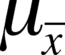) should = . This can be derived most simply through some logical argument. If random chance is the only reason a sample mean differs from , then all of the s should be clustered around and when you take their average, the random errors should about cancel out, making the expected average of the sample means the true mean.
  • This implies that, random chance will be as likely to increase a sample mean (compared to the true mean) as to decrease it
  • This also implies that (about) half of the sample means will be larger than the true mean and half will be smaller
• The "about" in the above statement arises from two sources: random chance is not precise but probabilistic and some of the sample means might equal the true mean

What is the expected standard deviation of these sample means?

• The standard deviation of sample means (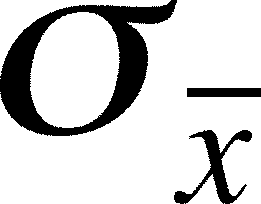.) must be related to the variation found in the original population, which is characterized by the population standard deviation, , but it is not simply equal to.  
• Why is this? 
  • Well, in the original population, the values of x had some range from the smallest to the largest and we use the standard deviation to characterize this variation.
  • The values of the means of samples will also have a range but is that range likely to be as large as the range of individual values in the population?
    • The difference is that the variation among the sample means should be smaller than the variation among the x values.
    • Each sample mean, , is calculated from a sample drawn from the population and will have the effect of some small and some large values.
    • For this reason, a sample mean, , from a randomly drawn sample should usually be closer to , the population mean, than an individual observation drawn at random from the population.
  • So, the sample means s cluster closer together, near , than do the members of the population, so their standard deviation, , should be smaller than the population standard deviation,
• But how much smaller?
  • Sample size is important once again.
  • Larger samples should estimate more closely, that is, the sample means, , from larger samples should be closer to than sample means calculated from a smaller sample.
  • If large-sample s are nearer one another (and ) then their standard deviation should be smaller.
  • So we need a way to reduce the population standard deviation, , to get the standard deviation of the sample means, , and that method has to make a larger reduction for big n's (sample sizes) than for smaller n's.
• Our solution:
  • Standard deviation of the sample means  =      =  /

What is the shape of the distribution of sample means?

The shape of the distribution depends on

• the shape of the distribution of observations that make up the population from which samples are drawn
• the sample size

These effects can best be summarized as below:

• When the population is normally distributed, the distribution of sample means for samples drawn from that population is also normal, no matter the size of the sample.
• When the population is not normally distributed, then the shape of the distribution of sample means depends on sample size
  • If the sample size is small (n about 40 or less), then the distribution of sample means for samples drawn from the population will not be normal (it will be similar to the population distribution)
  • If the sample size is large (greater than 40 or so), the shape of the sampling distribution of sample means will be normal, no matter whether the population is normally distributed or not - this is due to the Central Limit Theorem, covered next
• Thus, problems with normality arise only when the sample size is small and the population the sample is taken from is not normally distributed

Central Limit Theorem

The distribution of the population has in influence on the distribution of s only when the sample size is small.

• As the sample size increases, the distribution ofs becomes closer and closer to a normal distribution, no matter what the population's distribution is.
• This is a very good thing for two reasons.
• First, it lets us use the same methods for drawing inferences about sample means no matter how skewed or kurtotic the original population distributions are. This makes things simpler than a different methodology for each distribution
• Second, we know lots of properties of the normal distribution and can make powerful inferences based on these properties
• However, notice that this is only true for large sample sizes
• We will see that this means that we need to approximate the normal distribution, and that the approximation should get closer to the normal as sample size goes up.
• We will do this in the next chapter.

So far we have three groups of numbers to keep track of. Here is a summary of the three (the book does this in Table 5.7)

1. The population of x's has a mean of and a standard deviation of
2. A sample of size n drawn from the population has a mean of and a standard deviation of s
3. Sample means (), each calculated from each sample drawn from the population have a mean of , which is expected to be the same as the population mean,, and a standard deviation of   which can be calculated directly as /

Normal Approximation of the Binomial Distribution

This section is another outcome from the central limit theorem.

Once again, the binomial has three parameters, Pr{a success for any particular trial} = , j = the number of success, and n = sample size or number of trials

If n is large, then the binomial distribution of outcome probabilities can be approximated by a normal distribution with (notice that I use p in this section and the book uses p, but these are the same value - I want to be more consistent)

• mean = n
• standard deviation = sqrt[n(1-)]

If n is large then the distribution of the probabilities of success () in the samples can be approximated with a normal distribution with:

• mean(p-hat) =
• standard deviation of p' = sqrt[(1-)/n]

Note the difference between the first and second set of means and standard deviations just presented!

• The first refer to the probability of getting j successes out of n trials (so the x-axis of the distribution will go from 0 to j in whole number jumps - remember it's categorical data)
• The second refer to the probability that the proportion of success in the n trials will be j/n (so the x-axis of the distribution will be a fraction from 0 to 1)

Why is this useful? Its a time saver when n gets large

• if n = 200, then what do you need to calculate the chance of getting more than 50 successes?
  • You have to calculate all of the binomial probabilities for 51 through 200 successes and sum these up.
    • or
  • You have to calculate all of the binomial probabilities for 0 through 50 successes, sum these up, and subtract the sum from 1
• That's lots of work.
  • With the normal approximation you have to calculate the mean and standard deviation, z-ify 50, and look up the area associated with that z in the normal table and subtract that area from 1

How large is large enough for the size of samples when deciding if the normal approximation will be close to the real distribution?  Below are reasonable guidelines (but they are arbitrary).  Note that we consider whether or not p-hat is close to 0.5 (central) or closer to 0 or 1.0 (the extreme values for )

• if ~ 0.5, then n can be as low as 10 or so
• if is close to 0 or 1.0, then if n* ~ 5 or if sqrt[n(1-)] ~ 5, the n is large enough

Continuity Correction

Note that, the binomial is discrete (and is represented by a histogram) and the normal is continuous and is represented by a curve.

This means that a continuity correction is called for, especially when n is small

• First, draw a histogram to depict the binomial probabilities and then draw a normal curve that approximates it
• Determine which binomial probabilities are of interest
• then add or subtract one half to the j values you are working with
• whether you add or subtract depends on the situation and which part of the end histogram bars are missing (assume that the normal values split the end bars in half)
• the addition or subtraction should be done to increase the final area under the normal curve

Last updated September 26, 2012