| Handout on Rarefaction Calculation
|
BIOL
4120
Principles
of Ecology |
 |
 |
 |
 |
 |
 |

|
Harned Hall 301 (615) 963
- 5782
|
| |
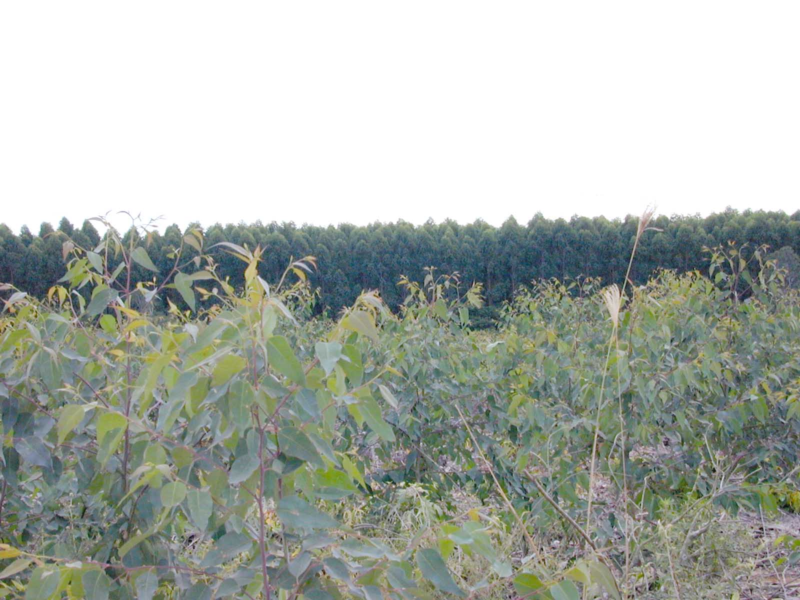
| Above: Young Eucalypt trees from Australia
growing in Brazil to provide fiber for disposable diapers. The newly
planted trees are in the foreground and the dark green band behind
them is the forest after only 5 years! Vast fields of eucalypts have
replaced the native ecosystem, the Atlantic Forest, one of the most
diverse and threatened of all terrestrial ecosystems.
|
Rarefaction
(From Lecture 16)
- Correction for bias in species
number due to unequal sample sizes by standardization to
the number of species expected in a sample if it had the same total size as
the smallest sample
- very similar to the idea behind Effective
Population Size for comparing genetic drift in two populations with different
mating systems or different histories
- Say you had two samples, A with
100 individuals total and those 100 individuals distributed among 9 species
and sample B with 25 individuals distributed among 4 species.
- Rarefaction answers the question
"How many species would I expect in sample A if I had caught only
25 individuals in all instead of 100?"
- N = total number of individuals
in rarefied sample (100 in the sample above)
- Ni = number of individuals
in the ith species
- n = size of the smaller sample
(25 in the example above).
- We want to calculate E(S),
which is the expected number of species
in the sample IF THE SAMPLE WERE OF THE SMALLER SIZE (n).
- Look at this expression and simplify it in
your mind. Each term that you sum is 1 minus a fraction, so each term you
sum is less than 1. You are summing up S (= number of species in the sample)
terms, so the sum will have to be less than S (since each term is less than
one and there are S terms). Therefore, the expected number of species will
be less than the actual number of species
- This is because you would expect to capture
fewer species in a smaller sample. The rarer species have less
of a chance of being taken.
- The expressions within the
inner most parentheses are not fractions, they are combinations
(note that there is no horizontal bar and see a discussion of combinations
in Lecture 13 from BIOL 3110,
my biostats class). These combinations are defined as:

- remember that the fraction
on the left of the = sign is not a fraction (note: no horizontal bar), and
the fraction on the right is one. The ! means that the expression is a factorial.
The expression on the left is called a combination because it gives you
the number of ways to take N objects n at a time. For instance, there are
three ways (= 3!/2!1!) to group 3 objects 2 at a time (1&2, 1&3,
2&3). Factorials (indicated by !) are gotten by multiplying the number
times one less times two less times ...
- What you are calculating in
the combinatorial expression found in the numerator of the fraction within
the summation in the top equation is the number of combinations one can
make (of the same size as the smaller sample size, n) without any of the
species of interest present (this is why we use N - Ni and not
Ni here). The total number of combinations possible is
calculated by the combinatorial expression in the denominator. This
fraction is then the proportion of combinations (each one represents a possible
sample) that contain none of the species of interest (species i).
This can be seen as the probability of not getting that species in the sample
and this fraction is subtracted from 1.
Without rarefaction, one can not
compare samples that have different number of individuals in each sample
Calculating Rarefaction
Remember that
# of Fish from three lakes |
| Species
of fish |
North America |
Central America |
Argentina |
|
A |
12 |
|
|
B |
5 |
|
|
C |
4 |
33 |
|
D |
3 |
32 |
|
E |
1 |
34 |
|
F |
|
33 |
|
G |
|
|
42 |
H |
|
|
23 |
I |
|
|
16 |
J |
|
|
14 |
K |
|
|
6 |
L |
|
|
5 |
| |
|
|
|
| total |
25 |
132 |
106 |
=N |
| each cell is an Ni |
| # of species
|
5 |
4 |
6 |
=S |
To compare all
three lakes, we need to rarefy the samples from Central America
and Argentina to the smallest sample, North America
The book does not say,
but n must be THE SMALLEST SAMPLE SIZE
The
criterion is that N > n, or you will not be able to do the
combinatorials when N < n
Therefore,
rarefaction always adjusts down, never up.
So, we can only ask
"How may species would I have gotten in this sample if it
had been as small as the smallest sample?
We will use n = 25
from the North American A sample and rarefy the North American B
and Argentine samples
Central America |
| |
N |
n |
Ni |
N-Ni |
N-Ni n
Factorial |
N n Factorial |
fraction |
1--fraction |
C |
132 |
25 |
33 |
99 |
1.82E+23 |
6E+26 |
0.0003 |
1 |
D |
132 |
25 |
32 |
100 |
2.43E+23 |
6E+26 |
0.0004 |
1 |
E |
132 |
25 |
34 |
98 |
1.36E+23 |
6E+26 |
0.0002 |
1 |
F |
132 |
25 |
33 |
99 |
1.82E+23 |
6E+26 |
0.0003 |
1 |
| |
|
|
Total = |
4 species |
In the Central
American lake sample, we do not get much of a correction (too
small to show up). Why?
- This sample is
very even, and if you reduce the sample size, all four
species should be sampled, as all are about equally
likely to be sampled
This situation is a
bit different for the Argentine sample, where the sample is not
so even, although the richness is greater.
Argentina |
| |
N |
n |
Ni |
N-Ni |
N-Ni n
Factorial |
N n Factorial |
fraction |
1--fraction |
G |
106 |
25 |
42 |
64 |
4.01E+17 |
1E+24 |
3E-07 |
1 |
H |
106 |
25 |
23 |
83 |
1.08E+21 |
1E+24 |
0.0008 |
1 |
I |
106 |
25 |
16 |
90 |
1.16E+22 |
1E+24 |
0.0091 |
0.99 |
J |
106 |
25 |
14 |
92 |
2.2E+22 |
1E+24 |
0.0172 |
0.98 |
K |
106 |
25 |
6 |
100 |
2.43E+23 |
1E+24 |
0.1902 |
0.81 |
L |
106 |
25 |
5 |
101 |
3.22E+23 |
1E+24 |
0.2528 |
0.75 |
| |
|
|
| Total = |
5.53 species |
Here, there is a
noticeable correction. Why?
- The less
common species are much more rare than are the most
common, and so, they might not be sampled at all in a
smaller sample.
The last example rearranges the
Argentine data, but keeps the number of species (6) and total sample size the
same (106). What it does is make species G more dominant at the expense of all
other species (look at the Ni column here and compare with the previous Argentina
table).
| Argentina
- with almost all fish from species G |
| |
N |
n |
Ni |
N-Ni |
N-Ni n
Factorial |
N n Factorial |
fraction |
1 - fraction |
G |
106 |
25 |
80 |
26 |
26 |
1E+24 |
0.00 |
1.00 |
H |
106 |
25 |
9 |
97 |
1.01E+23 |
1E+24 |
0.08 |
0.92 |
I |
106 |
25 |
7 |
99 |
1.82E+23 |
1E+24 |
0.14 |
0.86 |
J |
106 |
25 |
5 |
101 |
3.22E+23 |
1E+24 |
0.25 |
0.75 |
K |
106 |
25 |
3 |
103 |
5.64E+23 |
1E+24 |
0.44 |
0.42 |
L |
106 |
25 |
2 |
104 |
7.42E+23 |
1E+24 |
0.58 |
0.24 |
| |
|
|
Total = |
4.50 species |
I included this
example for two reasons
- Reason 1 -
notice that the effect here is much more drastic because
the community is much less even. Now, you expect to get
only 4.18 species when you sample only 25 individuals.
- Reason 2 - Suppose that the number
of species G was 82 (and there were two less of Species K, to keep the total
the same). When you calculate this rarefaction, you run into an impossible
situation. The combinatorial in the numerator for species G is impossible
to calculate. It is 24 over 25. You can't calculate this, because it becomes
The -1 from the ((N - Ni) - n)
factorial (from 24 - 25) is the problem. You must set this combination
to 0 to do the calculations in the rarifaction table because the combination
(24 over 25) means you want to calculate the number of combinations of 25
objects one can make with only 24 objects to combine! Obviously, there
are no combinations possible and the answer is 0. When doing these calculations
in a spreadsheet, the program will return some sort of error code for any
situation in which you have asked for the factorial of a negative number.
Whenever this occurs, simply set the value of the calculation at 0 and proceed
with the calculations.
So, we see that rarefaction
is a bit more involved than the text makes out, but still a necessary exercise
when making comparisons of species richness among samples that differ in size.
In
addition, honesty makes me disclose that this is not the only way
to rarefy a sample
For example, one might
use a bootstrap approach (made possible by the speed of computers)
In this approach, one
subsamples a larger sample repeatedly and then calculates the parameter
of interest based on the subsamples
- For the above example comparing the Argentine
lake with the North American lake, one would make a subsample by taking
the 106 individuals in the larger sample and randomly choosing only 25
of the 106 to be in the subsample. One would then count the number
of species in the subsample and that would be one bootstrap estimate for
species richness.
Next, one would resample
the original 106 individuals again, choosing another 25 at random (some
of those in the second subsample could have been in the first) and recalculate
the number of species.
Repeat the subsampling
many times (this is why a computer is necessary, 10,000 is a good number
of subsamples), each time getting an estimate of the species richness.
Finally, average the
10,000 richness values for the 10,000 subsamples and use that average as
your rarefied estimate of richness [ = E(S) in the formula above].
The bootstrapping approach supplies an additional bit of information.
One can do the bootstrap estimate for any subsample size and graph the expected
number of species in the sample versus the sample size. This is a Rarefaction
Curve and it usually has a steep portion before it plateaus
as the subsample size approaches the larger sample size. If your smaller
sample is in the plateau region, the two samples are reasonable compared.
If not, your smaller sample most probably is deficient as a sample of the diversity
(compared with the larger sample).
Last Updated on July 23, 2007