 |
BIOL 3110
Biostatistics Phil Ganter 301 Harned Hall 963-5782 |
The star-like plants among the ferns are Ground Pine, Lycopodium, very ancient plants |
|
| |
BIOL 3110
Biostatistics Phil Ganter 301 Harned Hall 963-5782 |
The star-like plants among the ferns are Ground Pine, Lycopodium, very ancient plants |
|
Introduction to Comparing Many Means
Chapter 11, part A
Back to:
This is the first part of a two-part set of lecture notes. The second part can be found here
Unit Organization
Problems
Problems for homework
- 3rd Edition - 11.1, 11.3, 11.6, 11.8, 11.13, 11.40, 11.42, 11.50
- 4th edition - 11.2.1, 11.2.3, 11.2.6, 11.4.1, 11.4.6, 11.S.1, 11.S.3, 11.S.12
Problems for homework
- 3rd Edition - Do at least 1 additional problem in each section covered by this lecture
- 4th edition - Do at least 1 additional problem in each section covered by this lecture
Basic One-Way Analysis of Variance
Many experiments involve more than a simple dichotomous "control vs. treatment" design.
Most have more than one treatment level.
How do we compare multiple samples at once?
We could do pairwise t-tests to see which differed from one another.
However, the
-level probability of making an error applies to each test, not to the series of tests.
So, the real chance of making a type I error is increased by using multiple tests.
There are ways of dealing with this, but it is time-consuming to do many pairs.
The analysis of variance procedure (called ANOVA) is a way to make multiple comparisons.
H0 : ![]() 1 =
1 = ![]() 2 =
2 = ![]() 3 = ....
3 = ....![]() n, for n means
n, for n means
HA : at least one mean is not equal to the others
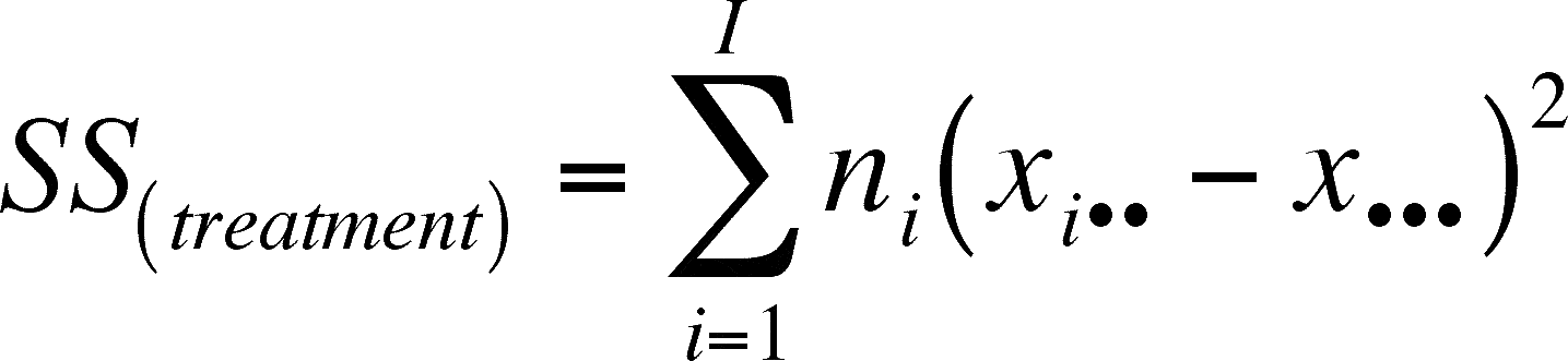
Some necessary definitions and notation
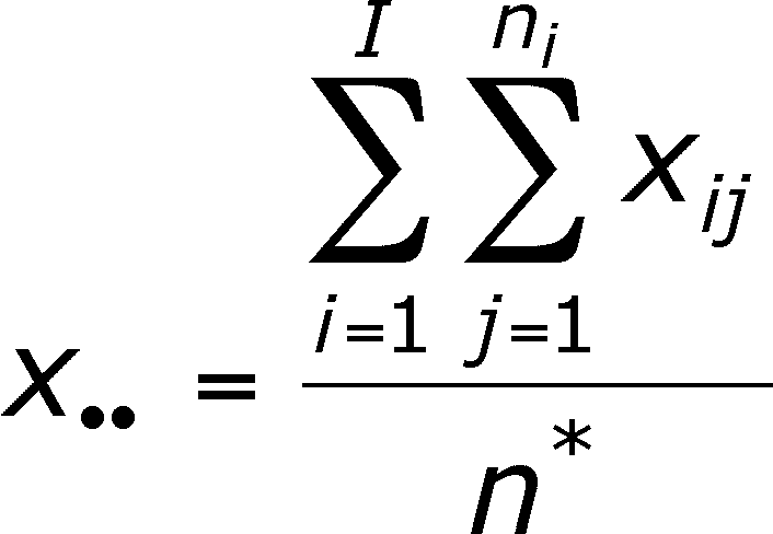
xij = observation j in group i
I = the number of groups
ni = the sample size of group i
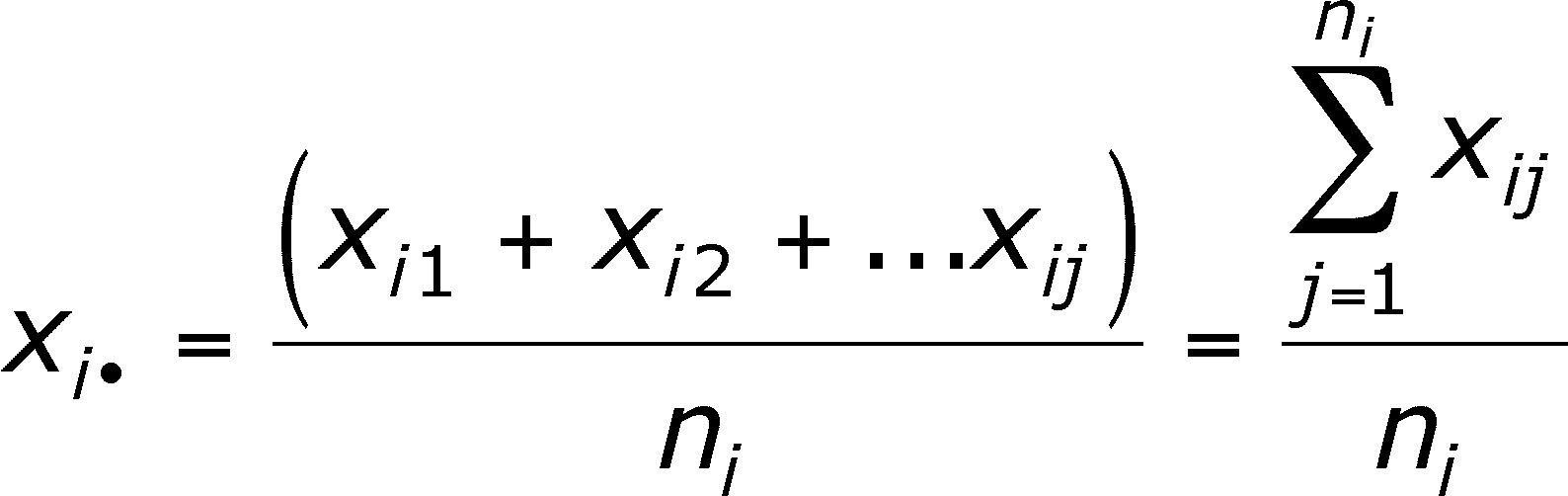
Dot notation = a dot that replaces an index stands for the mean for the observations the dot replaces.
xi• = mean for group i (the j's have been averaged for the group)
In summation notation, the dot looks like:
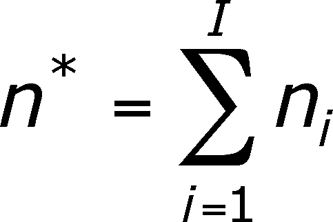
The total number of observations is:
DOUBLE SUMMATION - two summation symbols in tandem indicates double summation.
This is done by doing what is instructed by the second (right side) summation for observations 1 to ni in group ni, then repeating that for each of the I groups and summing each sum into a grand total.
Below, double summation is used to get the mean of all of the observations. The right hand summation gets the sum of the observations within each group and the left summation sign gets the sum of the sums of each group.
This is the grand total, which is divided by the total number of observations, which is the definition of a mean! Look at the formula below. I will call this the OVERALL MEAN
Now we need to define some of the terms that will be important for this technique (before we cover the technique itself).
The first term is called a "SUM OF SQUARES" (abbreviated "SS"), which is more than just the sum of some squares. Before you can sum, you must correct the observations for the mean of the group to which they belong, then square that difference before summing up the squares (it is often said that the squares have been "corrected for the mean").
SUM OF SQUARES: TOTAL, WITHIN GROUPS, AND BETWEEN GROUPS
SS(total) means the sum of squares for all of the data, corrected for the OVERALL MEAN OF ALL OBSERVATIONS. The formula below is a double summation. The first (right-side) summation tells you to subtract the overall mean from each member of group i and square the difference. You then sum the squared differences for each member of group i to get a group sum. Do this for each of the i groups. The second (left-side) summation tells you to sum the sum-squares for each of the groups. Notice that each group has been corrected for the overall mean of the data.
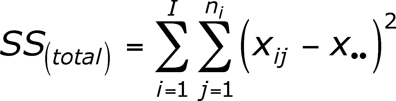
So, what have you calculated? You have subtracted the overall mean from each observation, squared the difference, and summed up all of the squares. This is a (kind of) measure of how much difference there is between the data and the overall mean (not an average difference but a total for all observations). If the observations are far from the mean, SS(total) will be large and if the observations are all close the mean, SS(total) will be small.
There are degrees of freedom associated with the total SS(total). If you were to look at all observations in a study as though they belonged to a single group, then SS(total) would be in the numerator of the variance formula (Chapter 2). And the denominator would be the total number of observations minus 1. This denominator is the degrees of freedom associated with the total
D. F. total = n* - 1
SS(within groups) means the sum of squares for all of the groups, corrected for the MEAN OF EACH GROUP. The formula below is again a double summation. The first (right-side) summation tells you to subtract the mean of the ith group from each member of the group and square the difference. You then sum the squared differences for each member of group i to get a group sum. Do this for each of the i groups. The second (left-side) summation tells you to sum the sum squares for each of the groups. Notice that each group has been corrected for its own mean (the group's mean), not for the overall mean of the data - as we did above.
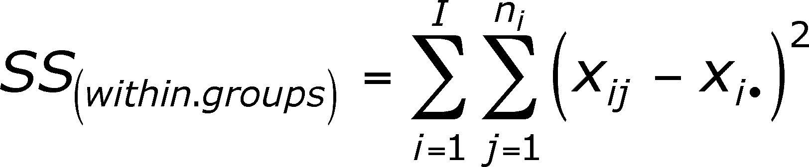
[NOTE FOR 4TH EDITION USERS ONLY -- If you are looking at the 4th edition of the book, you should note that their equation for SS(within groups) on page 422 differs from the formula above. The authors of the book apparently feel that students can not comprehend double summation and have chosen to use a rather unusual means of avoiding it (I can find only one instance where they use it on page 420.) I feel that their approach makes ANOVA a mystery by hiding the actual calculations and that, if you follow it, you will only learn the procedure as a recipe and won't understand the numbers you are calculating. In fact, the two formulas are equivalent. I will demonstrate this in class and discuss why their approach is deficient at that time.]
How does SS(within groups) differ from SS(total)? SS(total) is a (sort of) measure of how much the data differs from the overall mean but SS(within groups) is a (sort of) measure of how much the observations differ from their group means. Remember that each group consists of observations undergoing the same level of the experimental (or explanatory) variable. If observations in one group differ in some consistent way from observations in other groups, then a group mean should be more similar to the observations in the group than the overall mean is to those observations. After all, the overall mean is calculated from all of the data and not just the group observations. So, SS(within groups) should be smaller than SS(total), IF the observations within groups are consistently different from observations in other groups (that is, if the experimental levels had an effect). By the way, the SS(within groups) can't be larger than SS(total)!
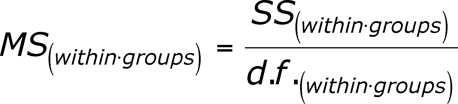
The third quantity to define is called a MEAN SQUARE, which is easy to calculate. It's just the SS(within groups) divided by the degrees of freedom for "within groups". This quantity is also easy to calculate. It's the total number of observations (n*, defined above) minus the number of groups (I).
DF(within groups) = n* - I
The mean square is then just =
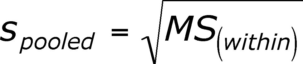
The mean square within groups is a combination of the variances of all of the groups and so it can be used to calculate a pooled standard deviation of the data=
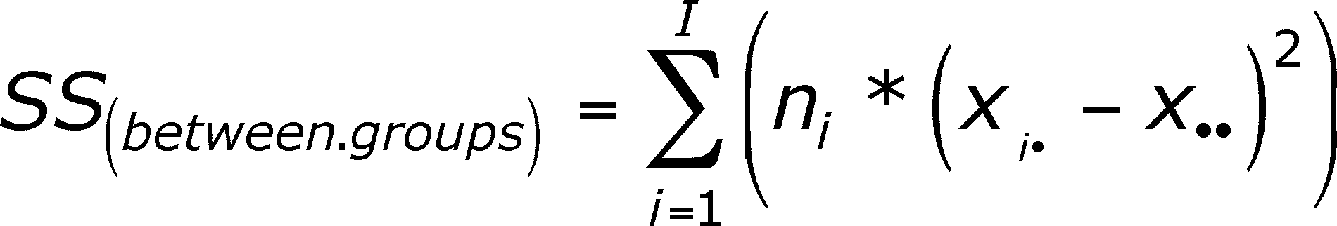
The "within groups" SS and MS refers only to the variation that occurs within the groups. This is the variation observations have from their group mean. Since SS(within groups) is smaller than SS(total), some SS is left over if you subtract SS(within groups) from SS(total). What does the SS left out represent? The difference between SS(within groups) and SS(total) represents the differences in the observations that are due to the effect of the experiment. The left over SS are due to each level of the experimental variable causing some consistent change to the observations experiencing that level. So, how do we calculate this portion of SS(total)? One way is to simply subtract SS(within groups) from SS(total). However, we can calculate it directly as done below (the subtraction is always an option).
The SS(between groups) is not a double summation. First, take the difference between each group mean and the overall mean. Square the differences. Multiply each squared difference by the number of observations in the group. Then sum these terms (there is one for each group).
There is a mean square for the between-groups variation, which is =
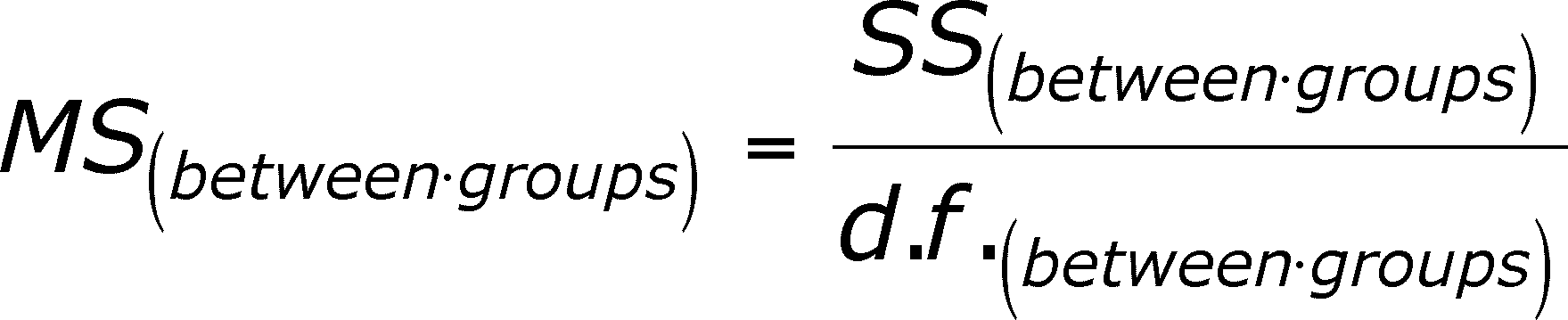
The degrees of freedom for between groups is the number of groups (I) - 1 (= I -1).
We can formalize the relationship between the Sum of Squares we have just calculated:
SS(total) = SS(between groups) + SS(within groups)
Another way to write this (in terms of an experiment) is:
SS(total) = SS(treatments) + SS(random error)
LOOK AT THESE EQUATIONS. THEY HAVE IMPORTANT IMPLICATIONS.
If we have a group of observations that have some set (= fixed) amount of variation among themselves, we have now PARTITIONED that variation into two groups.
The within group partition is the variation associated with differences among members of a group. This is the differences among the observations in the control group or the differences among the observations within each of the treatment groups (however many treatment groups there are).
The between group partition is the variation associated with being in different groups.
If SS(total) is fixed (= can't change), then as SS(treatments) increases, SS(random error) must decrease.
A successful experiment has most of the sums of squares in the between group partition, so that groups differ (treatments differ from control, etc.).
An unsuccessful experiment has most of the sums of squares in the within group partition, so that it doesn't matter which group an observation is in (treatment means are the same as control, etc.).
This is the key to understanding why ANOVA is such a useful technique.
Let's go to a simple example. We will use nine observations grouped into three groups.
First grouping:
Group 1 = 2, 5, 9
Group 2 = 2, 5, 9
Group 3 = 2, 5, 9
Where is the variation in this data? There is variation within each group, but the groups all have the same mean and the same observations, so there is no variation between the groups.
What if this were an experiment in which the first group was a control and the groups 1 and 2 were two treatment levels?
There is no chance of rejecting the null hypothesis here. The treatments did not differ from one another or from the mean in their effect. The groups are all identical and the experiment failed to influence the observations.
In terms of sums of squares, all of the SS are in the within-group SS and none is in the between-group.
Now lets re-group for a second example where we use the same data, but rearrange the groups:
Group 1 = 2, 2, 2
Group 2 = 5, 5, 5
Group 3 = 9, 9, 9
Notice that all of the observations are still here (three 2's, three 5's and three 9's).
If you calculate the SS(total) of this data, it will be exactly the same as in the first example above (try it!).
Where is the variation in the data now? There is no variation within each group, but the groups have different means so there is variation associated with the differences between the groups.
What if this were an experiment in which the first group was a control and the groups 1 and 2 were two treatment levels?
Now you have an effect of the treatments, which even differ from one another.
In terms of sums of squares, all of the total SS is in the between-group SS and none is in the within-group SS.
The book has a short section on the more formal model for ANOVA, which is worth a look. It's only slightly different from the interpretation above.
The basic model says that any observation, xij, is the sum of three things: the overall mean, the effect of being in group i, and the effect of random error within group i.
If we let tau (
) symbolize the group membership effect and epsilon (
) the random error effect, then
xij = ![]() +
+ ![]() i +
i + ![]() ij
ij
or, if we use our estimates of these population values
xij = x•• + (xi• - x••) + (xij - xi•)
With this model, the null hypothesis is that all of the
It is useful to note here that the error term,
When we calculate SS(within) (and MS(within)) we are measuring the size of random error in the model. This will be useful to remember when we go to the section about evaluating the results of the ANOVA (in the global F-test section).
There is a standardized way of presenting the calculated values.
| Source | d f |
SS |
MS |
| Between Groups | I - 1 | SS(between groups) | MS(between groups) |
| Within Groups | n* - I | SS(within groups) | MS(within groups) |
| Total | n* - 1 | SS(total) | |
Note that the sum of the between and within d f's is the total d f (same for the SS column) and that we need not calculate a total MS. This is because our evaluation of this table depends on the ratio of within to between MS. The probability distribution of this ratio is the subject of the next section.
Now that we can calculate and ANOVA table, what does it mean?
Remember that we want to evaluate the null hypothesis of no difference between the group means.
This step normally means that we calculate a statistic, look that statistic up in a table of probabilities of getting a statistic that large or larger if the null hypothesis is true, comparing this probability (p) to the maximal acceptable risk of committing a type I error (the
No difference here.
But what is the correct probability distribution? It's not the z, t, chi-square, or binomial. We need a new distribution and this one was first described by a biologist who was also a statistician, Ronald Fisher
It is worth noting that Fisher's life-long work was population genetics. He was a statistician because he needed the tools of statistics to do his work but no one had invented those tools yet.
In honor of Fisher (who is also responsible for Fisher's exact test of last lecture), the probability distribution is referred to as the F distribution.
It is not symmetric, like the z or t, but it gets more symmetric as the degrees of freedom increase.
The statistic is simply
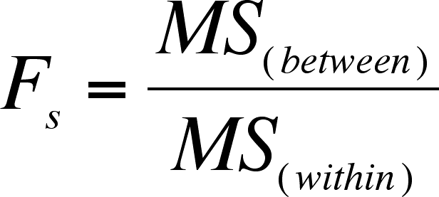
Note that each mean square has a degrees of freedom associated with it.
The df of the MS(between) is the numerator df = I - 1
The df of the MS(within) is the denominator df = n* - I
If you go back to the models for ANOVA, then you will realize that the F ratio is a ratio of variation due to group effect to the variation due to within group effect
We have already noted that within-group variation is the measure of random error, so the ratio is really the effect of the treatment to the effect of random error, which is what we want to test.
If random error is large and treatment effect is small, the ratio will be small and we will not be able to reject the null
If random error is small and treatment effect is large, then the ratio will be large and we are more likely to reject the null.
How to use the table
As usual, you look up your p-value (probability
of committing a type I error - of rejecting the null when the null is true)
and compare it with the already established ![]() -value.
-value.
To use the table in the book:
go to the page that lists the p-values for the numerator df (df for MS(between))
go down the page until you get to the df for the denominator (df for MS(within))
go across the page on that row until you find two columns that bracket your Fs
Look at the probabilities at the top of the columns that bracket your Fs. Your p-value is between those probabilities.
Relationship between F and t distributions
If you have only two groups and substitute the pooled s for the actual s, then calculate SE from this, then the two tests are equivalent.
For any set of data with two groups and n1 and n2 as the sample sizes,
the df for the t-test is n1 + n2 - 2, and the df for the equivalent F-test is (I - 1 = 2 - 1 = 1, (n* - I = n1 + n2 -2) - numerator df first, denominator second.
For any
Why the global in the section name? In a more complicated experimental design (with more than one treatment variable) there are more than one F-test that can be done.
Assumptions of the test
When can you apply this method?
The samples must be randomly taken from their respective populations.
This is checked by examining the methods used to sample.
Each sample must be independent of other samples.
This is checked by examining what is known of the two populations.
The populations must be normally distributed.
This can be checked by examining histograms of each sample or by using something like a normal probability plot.
The central limit theorem applies here, as well, so that, as sample size of each group increases, this assumption is relaxed more and more.
The populations must have equal standard deviations (or variances, which is how most authors choose to state this). This assumption is called HOMOSKEDASTICITY
This can be a problem and is often ignored.
One way to check for a problem is to plot group standard deviations versus group means. A positive trend can signal trouble.
Log-transforming the data before analysis can alleviate this problem. It compresses the range between the largest and smallest values.
The book recommends that the largest SD of any group be no larger than twice the size of the smallest SD, especially if the sample sizes are small and/or unequal.
A direct test of the equality of variances is found in Lecture 13
This is the simplest level of Multivariate ANOVA, or MANOVA.
Here we have a second treatment variable of interest.
What if we wanted to know if different sexes reacted to increasing levels of a drug?
What if we had to analyze blocks and experimental treatments?
As you can see, experimental design can become very complicated, which is why there are books and courses in experimental design. We will only cover some basics here.
Analysis with blocks as a variable.
Imagine an experiment in which the replicated treatment levels have been assigned to different blocks.
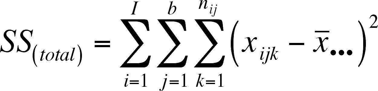
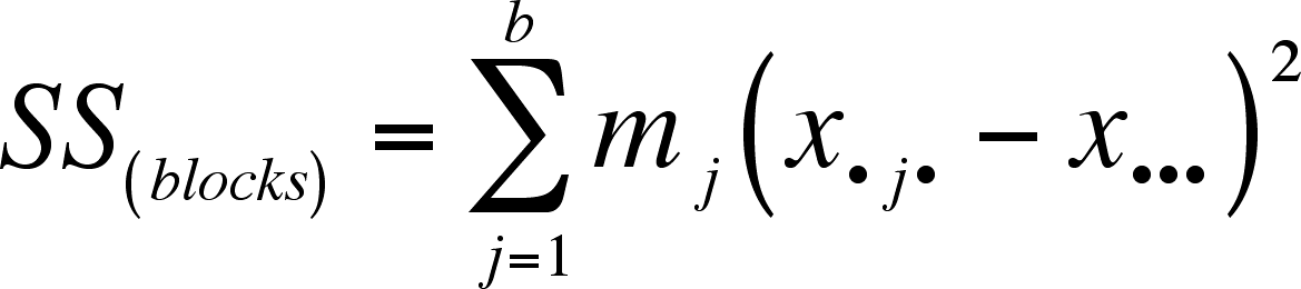
We now need three different indexes: i for different treatment groups, j for different blocks, and k for different observations within blocks. The number of blocks = b and block j has mj observations (=replicates) in it. As before, each treatment level has ni observations in it.
The mean of block j is x•j•, the mean of each treatment group is xi••, and the overall mean is now x•••.
We need to define the SS(blocks) SS(between), and SS(within) so that we can incorporate them into our calculations. Note that 'between' is now referred to as 'treatment' (the experimental manipulation) and 'within' as 'error'.
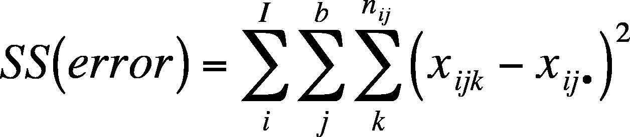
The way to get the SS(error) is to subtract both the SS(treatment) and SS(blocks) from SS(total)
SS(error) = SS(total) - SS(treatment) - SS(blocks)
The SS(error) is always calculated the same way - the mean for each treatment combination is subtracted from each replicate in that combination and squared, then summed over all observations. The formula below will work for our block situation. However, the easiest way to do get the SS(error) is by subtraction, as done above.
To specify the number of observations found in each combination of block and treatment, we need to double-index n, which becomes nij. For example, n3,.2 is the number of observations in the third level of the second block.
SS(total) is found in the original way - simply subtract the overall mean from each observation, square the difference, and sum the squares.
In this case, the SS(total) is being partitioned into three terms:
SS(total) = SS(treatments) + SS(blocks) + SS(error)
Since SS(treatments) is calculated in the same fashion and will not change, all of the SS(blocks) are being taken from SS(error) (SS(total) will not change).
Since we have the formulas for SS(total), SS(treatments), and SS(blocks), we can calculate SS(error) as the difference:
SS(error) = SS(total) - SS(treatments) - SS(blocks)
The df for the error term is also easiest if done by subtraction:
df = n* - I - b - 1
If you add the treatment, block and error dfs together you get n* - 1, as you should as you can' have more df in the model than you have for the total.
The model we will use is this:
Any observation, xijk, is the sum of four things: the overall mean, the effect of being in group i, the effect of being in block j and the effect of random error within group i and block j (the random error term is again the within-cell variation). Cells are combinations of
If we let tau (
the block effect, and epsilon (
xijk = ![]() +
+ ![]() i +
i +![]() j +
j + ![]() ijk
ijk
or, if we use our estimates of these population values
xijk = x••• + (xi•• - x•••) + (x•j• - x•••) + (xijk - xij•)
With this model, the null hypothesis is that all of the
What the model above does is remove some of the variation from the error SS, which will make it smaller and probably the error MS smaller, so the F ratio will probably be larger and we will be more able to reject H0, which improves the power of the test.
I say probably will make the MS smaller, because the blocks term removes some of the error SS but it also removes some of the error degrees of freedom, so the MS(error) will be smaller only if the blocking was effective.
The table for this is below (the MS terms = SS divided by the df, as before):
Source d f
SS
MS
Treatments I -1 SS(treatments) MS(treatments) Blocks b - 1 SS(blocks) MS(blocks) Error n* -I - b + 1 SS(error) MS(error) Total n* - 1 SS(total)
The F-value for treatments is once again MS(treatments) divided by MS(error), as before and is evaluated as before.
(Treatment effectiveness can be tested by looking at MS(blocks) divided by MS(error) and evaluating it like the treatment effect.)
Last updated October 28, 2011