BIOL 4120 Principles of Ecology Phil Ganter 302 Harned Hall 963-5782

Chapter 6 Population Growth

Email me

Back to:

Sections:

• Demography
• Life Expectancy
• Net Replacement Rate
• Generation Time
• Deterministic Models of Population Growth:
  • Geometric Population Growth
  • Exponential Population Growth
  • Logistic Growth
• Stochastic Models
• Terms

Descriptions of Populations:

Demography is the science of life tables

Life Tables are accounting of births and death in a population

Usually the life span of an individual is broken into stages (egg, larvae, etc.) or by age intervals or classes (0-5 years, 5-10, etc.)

Cohort - all of the individuals born at the same time

x = the interval

n_x = the number alive at the START OF THE INTERVAL

l_x = age specific survivorship -- fraction of cohort alive at the START OF THE INTERVAL

d_x = age specific mortality -- number dying in the interval

q_x = age specific mortality rate -- death rate for individuals of a specific age

e_x = age specific life expectancy - number of years left for an organism of a particular age. IT IS NOT ALWAYS MAXIMAL AT BIRTH!!

b_x = age specific natality -- number born in the interval

m_x = age specific birth rate - the per female rate of offspring production for females of a particular age.

R₀ = net replacement rate = the number of females alive in the next generation for each female alive in the present generation.

T = generation time -- the average time between a birth of a member of the cohort and the birth of a member's offspring

Age specific means that the parameter varies with the individual's age

By convention, the first age interval has the notation 0, so the number in the cohort at the start is n₀.

Another convention (especially for human life tables) is to multiply the number in the l_x column by 1000 (if it is actually 0.562, then it reads 562).

However, if you wish to calculate the net replacement rate (equation given below), then you must either convert l_x back to a proportion or you will be calculating the number of females in the next generation per 1000 females alive in the present generation!

If we plot log (nx) versus age, we can see where most of the mortality occurs by where the numbers drop

• Type I Mortality curve
  • most mortality comes late
  • characteristic of K-selected organisms (us)
  • often associated with organisms that put a lot of resources in to postnatal care
• Type II Mortality curve
  • mortality constant throughout life
  • results in a constant proportion of each age class surviving
  • birds are the classic example
• Type III Mortality curve
  • most mortality comes early
  • characteristic of r-selected organisms
    • many exceptions to this generality

Life Expectancy

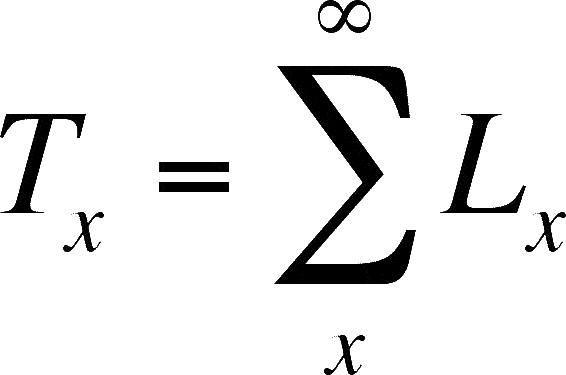
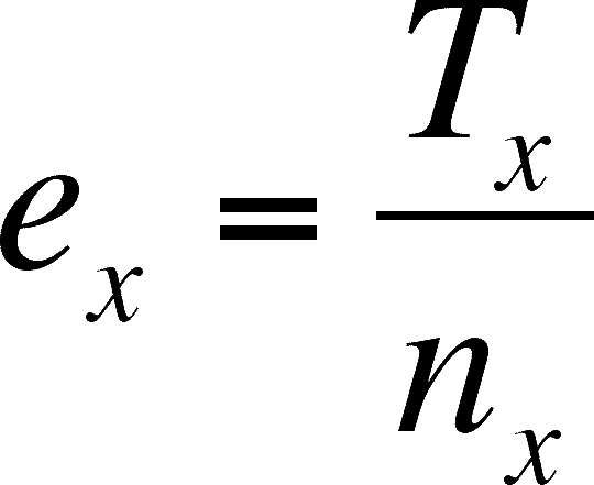
To calculate e_x, we will need to tack on another pair of columns to make it easier to do. This column is L_x, the average number alive in interval x. This is simple to do:

From this column, we can get Tx, which is the sum of all of the Lx values from x until the age that the last member of the cohort dies (this is symbolized by L°).

Life expectancy at age x is simply the average number of years lived by members of the cohort that are age x.

Net Replacement Rate

Net replacement rate is a measure of relative growth. It is the number of females alive in generation x+1 for each female alive in generation x. If it is greater than 1, the population is growing as there are always more females alive in the next generation than in the present. If less than 1, the population is decreasing (less than 1 female in the next generation per each alive in the present generation), and a net replacement rate of 1 means each female is exactly replaced in the next generation, so the population is stable, neither growing nor declining.

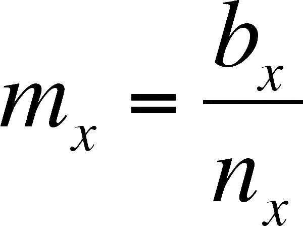
If we eliminate the males and add a column containing births, then we can calculate the net replacement rate. First, we must calculate the per capita birth rate (mx) for females of age x (females only!)

The net replacement rate is the sum of age-specific birth rates times the age specific survivorship. This means that an age class's contribution to the replacement rate must take account of the probability of surviving to that age.

The net replacement rate is a measure of population growth rate.

If it is 1, then the population in neither growing or declining in size (a stable population).

If it is less than 1, the population is declining by that proportion each generation (if it is 0.5, then the population will be half as big each generation).

A value over 1 indicates a growing population (a value of 2 is a population that doubles each generation).

Generation Time

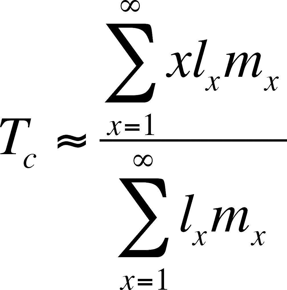
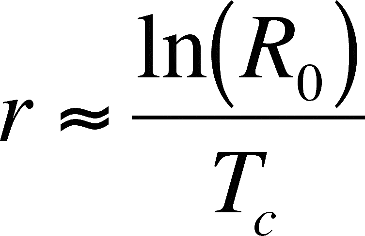
Assume that the net replacement rate is near 1. If so, we approximate the generation time as:

The approximation is due to the discrete nature of a life table, versus the continuous nature of time (an integral approach would get the exact figure)

Deterministic Models of Population Growth:

A model is a description of a natural phenomenon

Can be

• verbal (a story)
• pictorial (graphs)
• mathematical (equations)

Can be:

• Deterministic - exactly predicting the outcome
• Stochastic - giving a range of possible outcomes, with a probability of each occurring

Geometric (discrete generations) and Exponential (overlapping generations) Population Growth

Geometric Population Growth

• Non-overlapping generations (univoltine insects, annual plants, etc.) use discrete equations
• The change in size over a generation is:
  • 
• And the change over many generations is:
  • 
• N_t the population number after t generations, N₀ is the original population size

   

  Exponential Population Growth

  Populations with overlapping generations (us!) use continuous equations

• Overlapping generations means that births are continuous, so that dividing young into cohorts is purely arbitrary
  • humans (and many great apes) have overlapping generations as do many small mammals (rodents) and many invertebrates in non-seasonal environments
  • Many mammals in seasonal environments do not have continuous generations, as all young are born within a few weeks of one another during a particular season
• Continuous equations describe events that occur continuously (like births in a population with overlapping generations)
  • Calculus is best to describe continuous events
  • Matrix algebra often better when generations are discrete
• Predicting the future size of a population based on its current size and assuming exponential growth can be done with the following equation:
• 
• r is the intrinsic rate of natural increase and is an instantaneous rate, which the book points out is the difference between the instantaneous birth and death rates (r = b - d), and is a per capita rate (an average rate taken over all individuals in the population)
• we can approximate this as (approx. because gen. time is approx.)



• the rate of increase in the population (dN/dt) is dependent on two factors:
  • the intrinsic rate of natural increase, which is one individual's contribution to population growth and so doesn't tell what the whole population is doing
  • the population size (larger populations increase by more individuals)

  

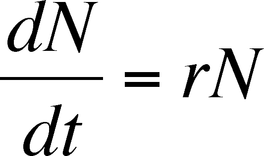
  The instantaneous rate of increase of a population (dN/dt) is the result

  For more on this topic, go to Modeling Exponential Growth page

Logistic Growth

In the last equation above, the rate of population increase simply increases with N

• Not very realistic, as all populations with an r greater than 0 would increase to infinity given infinite time
• Logistic growth is one way to limit the population size

Logistic growth is based on the idea of a Carrying Capacity (K) for any environment, a population size:

• Above which the population decreases
• Below which the population increases
• When the population size is at the carrying capacity, then no growth occurs

• If K is the carrying capacity in the environment (expressed in numbers of individuals of a species) then
  • 
• produces a sigmoid curve
• hits an equilibrium value
  • stable equilibrium because the population returns to it from any other population size, given time
• logistic growth model:
  • is a continuous model (notice that what is predicted above is the growth rate, not the size of the population
    • there is an equation, based on the logistic above, for predicting population size, but we will not use it here and so I will not present it
  • is useful because it is conceptually straightforward, although it does not accurately predict the growth of many natural populations
  • assumes that:

    1. the change in dN/dt with a change in N is linear
       • a graph with N as the X-axis and dN/dt on the Y-axis would be a straight line
       • for animals with complex life histories and mating systems, this assumption is not always met
       • social systems which entail some individuals not breeding when they could obviously violate this assumption
    2. there are no lags in the timing of the change in dN/dt with any change in N
       • lags are common when life histories are complex, as in holometabolous insects
         • larvae live in different environment and a change in larval density may not have an effect on egg-laying until after they pupate and become adults
    3. constant K (constant environment over space and time)
       • K is likely to change over both space and time
    4. constant r (all individuals equally fit)
       • often only a portion of a population breed, the rest may be helpers or may not have access to enough resources to breed
    5. no migration
       • dispersal can be important, even keeping a population from going extinct when the net replacement rate is below 1

• Time lags introduce oscillatory behavior into these models
  • populations can cycle between small and large values, with even intermediate levels possible
  • With lags, nonlinear relationships between dN/dt and N, and/or large r values, the models can become chaotic

For more on the logistic, including a derivation and some problems, go to Modeling Density-Dependent Growth

Stochastic Models:

Usually based on discrete models, but make allowance for the fact the things vary in the real world

Predictions of population size are couched as probability distributions

• X axis is the size of the population at some time in the future
• Y axis is the probability of the population being at some particular size

In general, the longer in the future you try to predict population size, the larger the range of possible sizes

Generalities:

Size and generation time are positively correlated (as one increases, so does the other)

Longer generation times are associated with lower intrinsic rates of growth

Terms:

Demography, Life Tables, Cohort, Age specific, age specific survivorship, age specific mortality, age specific mortality rate, age specific life expectancy, age specific birth rate, Type I, Type II, and Type III Mortality curves, Net Replacement Rate (R₀), Generation Time (T_c), model, verbal, pictorial and mathematical models, Deterministic and Stochastic models of population growth, Exponential (= Geometric) Growth, overlapping generations, continuous equations, intrinsic rate of natural increase (r), instantaneous rate of increase of a population (dN/dt), Carrying Capacity (K), sigmoid curve, stable equilibrium, logistic growth model, Time lags, chaos, deterministic and stochastic models

Last updated September 9, 2006